---------------------------------------------------
# #
# Chapter 3: Time Series Models with #
# Return-Driven Volatilities: #
# A Common Sense Approach #
# #
---------------------------------------------------
In chapter2 we took a closer look at the returns of liquidly
tradable financial assets. Recall the definition
ret(t_k) := (S_k - S_{k-1}) / S_{k-1} (1)
We summarized our results in the following
-----------------------------------------
# main conclusion chapter2: #
-----------------------------------------
The normalized returns
normret_d(t_k) = ret(t_k) / stddev_d(t_{k-1}) (2)
may be approximated pretty well by a standard normal distri-
bution, if the time horizon d is chosen not too large: d=15
days or d=20 days turned out to be quite reasonable choices.
Thus we can write
ret(t_k) / stddev_d(t_{k-1}) = phi_k (3)
with phi_k being a standard normal random number. Equation (3)
is equivalent to
S_k = S_{k-1} * [ 1 + stddev_d(t_{k-1}) * phi_k ] (4)
with the d-day standard deviation or volatility given by
[stddev_d(t_{k-1})]^2 (5)
= 1/d * [ret^2(t_{k-1})+...+ret^2(t_{k-d})]
-----------------------------------------
# end main conclusion chapter2 #
-----------------------------------------
Equation (4) allows the recursive calculation of the S_k's given
the data on day t_{k-1} and by drawing one random number phi_k.
Now, is this a reasonable stochastic model? Or more precisely,
why should it be not? Let's simulate a couple of paths with the
dynamics given by (4):
# Start R-Session:
#
# We name the model (4,5) the `naive ARCH Model' (apparently then
# there will be a non-naive ARCH-Model) and we code a function
# which generates a price path according to (4) for N time steps
# (for example N=2500 for 10 years = 2500 banking days):
pathNaivArch = function( N , d , startvol )
{
S = rep(0,N)
ret = rep(0,N)
phi = rnorm(N)
S0 = 100
stddev = rep(startvol,N)
summe = 0
for(k in 1:N)
{
if(k==1)
{
S[k] = S0*(1+startvol*phi[k])
ret[k] = (S[k]-S0)/S0
summe = summe + ret[k]*ret[k]
}
else
{
if(k<=d)
{
S[k] = S[k-1]*(1+startvol*phi[k])
ret[k] = (S[k]-S[k-1])/S[k-1]
summe = summe + ret[k]*ret[k]
if(k==d){stddev[k] = sqrt( summe/d )}
}
else
{
S[k] = S[k-1]*(1+stddev[k-1]*phi[k])
ret[k] = (S[k]-S[k-1])/S[k-1]
summe = summe + ret[k]*ret[k]
summe = summe - ret[k-d]*ret[k-d]
stddev[k] = sqrt( abs(summe)/d )
}
}#end if else
}#next k
plot(S,type="l",ylim=c(0,250))
return(S)
}
# If we put d = N, then for all time steps k only the constant
# startvol will be taken, thus in that case we simulate the
# model
#
# S_k = S_{k-1} * [ 1 + bsvol * phi_k ] (6)
#
# with bsvol = startvol a constant number which does not change
# during the simulation.
#
# `bsvol' stands for `Black-Scholes volatility' and the model
# (6) with a constant volatility is called the Black-Scholes
# model (here in discrete time). In 1997, F.Black, M.Scholes
# and R.Merton received the Nobel-prize for Economics:
# from nobelprize.org:
"Fischer Black, Robert Merton and Myron Scholes made a pioneering
contribution to economic sciences by developing a new method of
determining the value of derivatives. Their innovative work in
the early 1970s, which solved a longstanding problem in financial
economics, has provided us with completely new ways of dealing
with financial risk, both in theory and in practice. Their method
has contributed substantially to the rapid growth of markets for
derivatives in the last two decades. Fischer Black died in his
early fifties in August 1995."
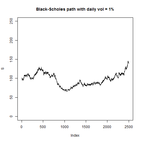
# Thus: the following command generates a Black-Scholes path
# for a time horizon of 2500 days or 10 years: d = N = 2500:
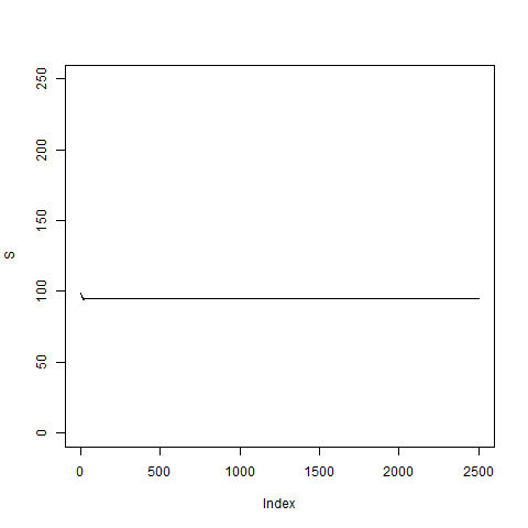
pathNaivArch(2500,2500,0.01) # looks ok so far.
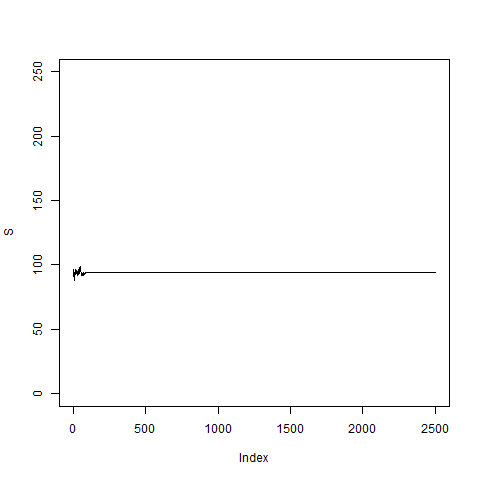
# now let's take a non-constant volatility, we use the realized
# volatility of the last, say, d = 20 days:

pathNaivArch(2500,20,0.01)
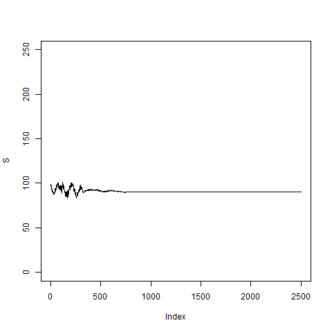
pathNaivArch(2500,20,0.02)
pathNaivArch(2500,20,0.03)
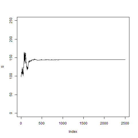
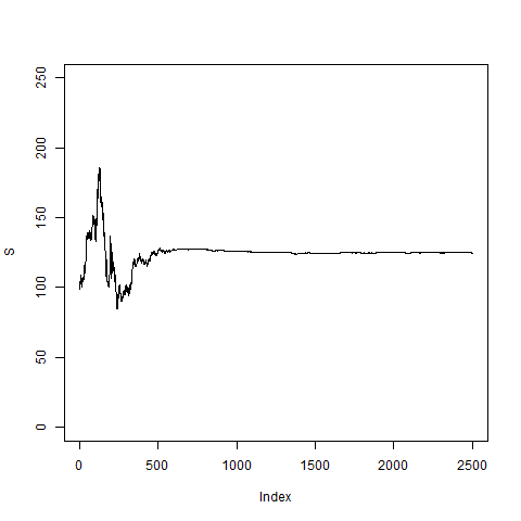
# now with d = 5 day volatilities:

pathNaivArch(2500,5,0.01)
pathNaivArch(2500,5,0.02)
pathNaivArch(2500,5,0.03)
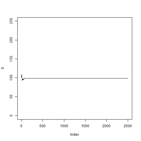
# Apparently this is not a good model; somehow the volatility
# goes to zero and then the price S_k stays fixed and does
# not move any longer.
# Let's make some theoretical considerations:


We had

ret(t_k) / stddev_d(t_{k-1}) = phi_k

or

ret^2(t_k) = phi_k^2 * [stddev_d(t_{k-1})]^2

with

[stddev_d(t_{k-1})]^2

     = 1/d * [ret^2(t_{k-1})+...+ret^2(t_{k-d})]

Thus:

ret^2(t_k) =

   phi_k^2 * 1/d * [ret^2(t_{k-1})+...+ret^2(t_{k-d})]       (6)


Let's consider d=1. In that case, we have:

ret^2(t_k) = phi_k^2 * ret^2(t_{k-1})
           = phi_k^2 * phi_{k-1}^2 * ret^2(t_{k-2})
           = ...
           = phi_k^2 * phi_{k-1}^2 * ... * phi_1^2           (7)

This expression is identical to the quantity pi_k
which we discussed in detail in the first three
exercise sheets and for which we found

pi_k ~ exp(-1.27*k)

Thus, for d = 1 the squared returns ret^2(t_k) converge
quickly to zero; for d > 1 we do no longer get such a
compact expression as in (7), but the mechanism, which
leads to the vanishing volatilities is basically the
same.

Thus, we have to make some adjustments to our model
given by (4,5) from above,

S_k = S_{k-1} * [ 1 + stddev_d(t_{k-1}) * phi_k ]            (4)

with standard deviations or volatilities

[stddev_d(t_{k-1})]^2                                        (5)

     = 1/d * [ret^2(t_{k-1})+...+ret^2(t_{k-d})]

This we will do in the next chapter 4.