---------------------------------------------------
# #
# Chapter 2: Typical Properties of #
# Financial Time Series #
# #
---------------------------------------------------
Returns of liquid tradable assets like stocks, stock
indices, currencies or commodities like oil, gold or
silver have some common typical properties which are
usually referred to as stylized facts. In the following
we list these stylized facts and illustrate them on
concrete data.
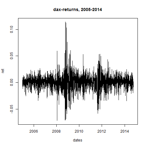
Let S_k denote the closing price of some liquid
tradable asset on day t_k. Its return ret(t_k) from
day t_{k-1} to day t_k is defined by
ret(t_k) := (S_k - S_{k-1}) / S_{k-1} (1)
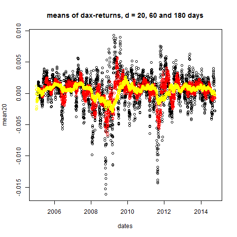
The d-day mean on day t_k is defined by
mean_d(t_k) := 1/d sum_{j=0}^{d-1} ret(t_{k-j}) (2)
There are the following so called stylized facts:
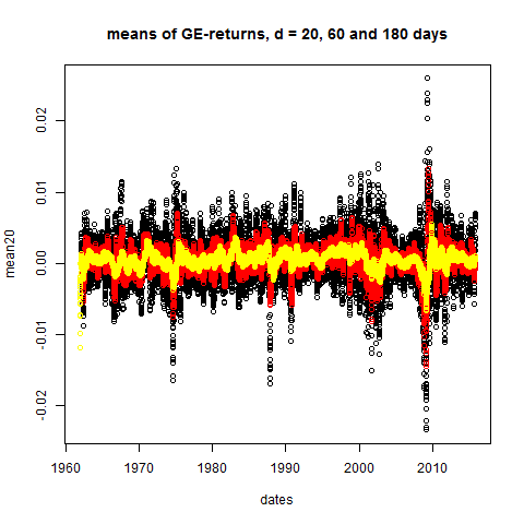
Stylized Fact 1) For arbitrary time horizons d (larger
than 2 or 3 weeks) the d-day means are close to zero.
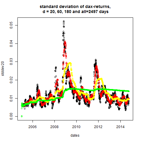
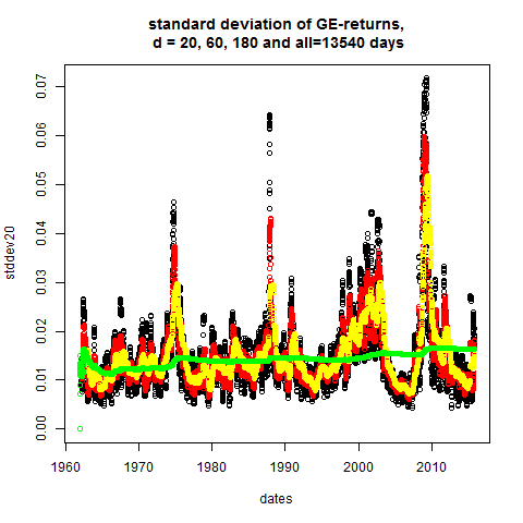
Because of stylized fact1 the d-day standard deviation
(also called d-day volatility) on day t_k can be defined
by
stddev_d(t_k) := sqrt{ 1/d sum_{j=0}^{d-1} ret(t_{k-j})^2 }
(3)
Normalized quantities, in a probabilistic context, are
defined by (quantity - mean)/stddev which reduces to
quantity/stddev if the mean is zero. Thus, because of
stylized fact1, we define normalized returns (for a
d-day time horizon) through
normret_d(t_k) := ret(t_k) / stddev_d(t_{k-1}) (4)
Then one can take a look at the distribution of the
normalized returns by making a histogram plot. One
finds:
Stylized Fact 2a) For large time horizon d (say, d>=250,
which corresponds to one year), the distribution of the
normalized returns is "leptocurtic", that is, there is
a more pronounced peak at zero and more faster decay
in a neighborhood of zero when compared to the standard
normal distribution. Furthermore there are "heavy tails":
there are some very large positive or negative normalized
returns which one would not see under the assumption of
a normal distribution.
Stylized Fact 2b) By making d smaller and finally put-
ting it to d=15 or d=20 (3 or 4 weeks), the distribution
of the normalized returns approaches more and more the
shape of a normal distribution. The occurance of heavy
tails decreases, but the variability of the d-day stddev
or equivalently, the variability of the d-day volatility
increases. This observation lies at the bottom of the
stochastic volatility models.
Furthermore one finds the following:
Stylized Fact 3) Returns for different days t_k are
nearly uncorrelated. However, the absolute value or
the square of returns have a significant positive
correlation (which could be around 10%-20%).
Stylized Fact 4) "volatility clustering": returns tend
to group themselves into clusters or phases with high
or low volatility, there is no uniform distribution
of the returns over time. This is also a motivation
for stochastic volatility models.
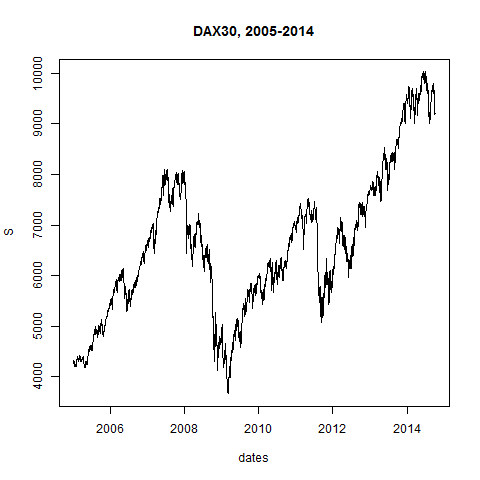
Let's demonstrate these facts now by looking at con-
crete data: the file DAX.txt contains the daily closing
prices for the time period 2005-2014, the file SPX.txt
contains the daily closings of the S&P500 for 1950-2015
and GE.txt contains the daily closing prices for the
General Electric stock from 1962 to 2015. This results
in approximately
DAX: 2500
SPX: 16500
GE: 13500
observation days. All data are taken from Yahoo Finance.
#
# Start R Session:
#
dax=read.table("C:/Users/Admin/Courses/FinancialStatistics/DAX.txt",header=TRUE,sep=";")
dax
head(dax)
tail(dax)
summary(dax)
str(dax)
# let's remove all rows with NAs:
dax = na.omit(dax)
summary(dax)
# in R there are basically 4 different data types: vectors,
# matrices, data frames and lists:
# dax is of type data frame
# the content of each column can be written into some vector:
names(dax)
S = dax$index # equivalent to S = dax[,2]
S
str(S)
plot(S)
plot(S,type="l")
dates = as.Date(dax$dates)
plot(dates,S,type="l",main="DAX30, 2005-2014")
S[1]
S[0]                      # vektor indices always start with 1, not 0
n=length(S)
n
S[n]
S[n+1]

# we calculate the returns:
ret = rep(0,n)            # vector of length n, all entries 0
for(i in 2:n)
{
  ret[i] = (S[i]-S[i-1])/S[i-1]
}
plot(ret)
plot(dates,ret,type="l",main="dax-returns, 2005-2014")
# we code 3 functions for the d-day means, stddevs and normrets:

dDayMean = function( d , ret )
{
  n = length(ret)
  result = rep(0,n)
  summe = 0

  for(i in 1:n)
  {
    summe = summe + ret[i]
    if(i > d)
    {
      summe = summe - ret[i-d]
      result[i] = summe/d
    }
    else
    {
      result[i] = summe/i
    }
  }
  return(result)
}

# let's take a look at Stylized Fact 1:
mean20 = dDayMean(20,ret)
mean60 = dDayMean(60,ret)
mean180 = dDayMean(180,ret)
plot(dates,mean20,main="means of dax-returns, d = 20, 60 and 180 days")
points(dates,mean60,col="red")
points(dates,mean180,col="yellow")
dDayStdDev = function( d , ret )
{
  n = length(ret)
  result = rep(0,n)
  summe = 0

  for(i in 1:n)
  {
    summe = summe + ret[i]*ret[i]
    if(i > d)
    {
      summe = summe - ret[i-d]*ret[i-d]
      result[i] = summe/d
    }
    else
    {
      result[i] = summe/i
    }
  }
  # a theoretical 0 could numerically become slightly negative:
  result = abs(result)     # we want to take a square root
  result = sqrt(result)    # square root element by element
  return(result)
}

# let's check:
stddev20 = dDayStdDev(20,ret)
stddev60 = dDayStdDev(60,ret)
stddev180 = dDayStdDev(180,ret)
stddev_n = dDayStdDev(n,ret)
plot(dates,stddev20,main="standard deviation of dax-returns,\n d = 20, 60, 180 and all=2497 days")
points(dates,stddev60,col="red")
points(dates,stddev180,col="yellow")
points(dates,stddev_n,col="green")
# apparently: volatility is not constant
dDayNormRet = function( d , ret )
{
  stddev = dDayStdDev(d,ret)
  # stddev could be 0 if data are constant:
  stddev = pmax(stddev,0.00000001)     # we want to devide by stddev
  result = ret/stddev                  # division element by element
  return(result)
}

normret15 = dDayNormRet(15,ret)
normret60 = dDayNormRet(60,ret)
normret250 = dDayNormRet(250,ret)
normret_n = ret/stddev_n[n]

par(mfrow=c(2,2),oma=c(0,0,2,0))       #set up 2 time 2 plot array
                                       #that is, 4 pictures at once
hist(normret_n,breaks=50,xlim=c(-5,5),ylim=c(0,0.8),prob=TRUE,main="d = 2497 (all days)")
curve(dnorm(x),from=-5,to=5,add=TRUE,col="red")
hist(normret250,breaks=50,xlim=c(-5,5),ylim=c(0,0.8),prob=TRUE,main="d = 250")
curve(dnorm(x),from=-5,to=5,add=TRUE,col="red")
hist(normret60,breaks=50,xlim=c(-5,5),ylim=c(0,0.8),prob=TRUE,main="d = 60")
curve(dnorm(x),from=-5,to=5,add=TRUE,col="red")
hist(normret15,breaks=40,xlim=c(-5,5),ylim=c(0,0.8),prob=TRUE,main="d = 15")
curve(dnorm(x),from=-5,to=5,add=TRUE,col="red")
title(main="Histograms of d-Day Normalized DAX30 Returns",outer=TRUE)

# thus: if returns are normalized with more recent volatility
# data, then normalized returns are more Gaussian.
#
# Heavy tails are less likely to occur, since the normalization
# can take care of a recent increase in volatility, if the nor-
# malization is calculated from more recent data instead of
# using the whole time horizon of 10 or 20 years.
----------------------------------------------
# let's redo this for SPX, since 1950: #
----------------------------------------------
spx=read.table("C:/Users/Admin/Courses/FinancialStatistics/SPX.txt",header=TRUE,sep=";")
head(spx)
tail(spx)
summary(spx)
str(spx) # no NA's!
names(spx)
S = spx[,2] # equivalent to S = spx$Adj.Close
dates = as.Date(spx$Date,format="%d-%m-%y")
dates # dates prior to 1969 have wrong year
datecorr = as.Date("1968-12-31") - as.Date("2068-12-31")
dates[1:4750] = dates[1:4750] + datecorr
dates
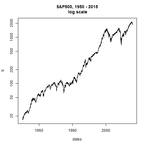
plot(dates,S,type="l",main="S&P500, 1950 - 2015\n linear scale")
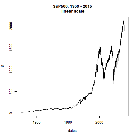
plot(dates,S,type="l",log="y",main="S&P500, 1950 - 2015\n log scale") # straight line would be constant exponential growth
n=length(S)
n
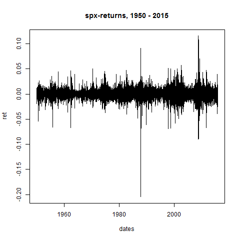
# we calculate the returns:
ret = rep(0,n)
for(i in 2:n)
{
ret[i] = (S[i]-S[i-1])/S[i-1]
}
plot(dates,ret,type="l",main="spx-returns, 1950 - 2015")
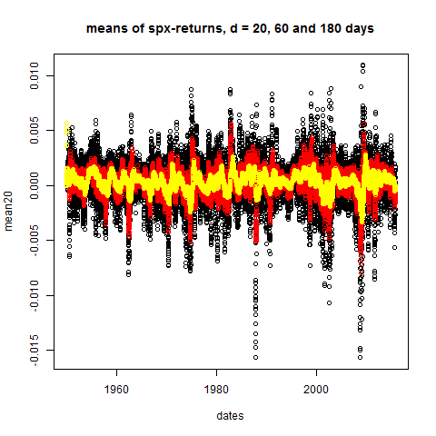
# let's take a look at Stylized Fact 1:
mean20 = dDayMean(20,ret)
mean60 = dDayMean(60,ret)
mean180 = dDayMean(180,ret)
plot(dates,mean20,main="means of spx-returns, d = 20, 60 and 180 days")
points(mean60,col="red")
points(mean180,col="yellow")
# stddev's = daily volatilities:
stddev20 = dDayStdDev(20,ret)
stddev60 = dDayStdDev(60,ret)
stddev180 = dDayStdDev(180,ret)
stddev_n = dDayStdDev(n,ret)
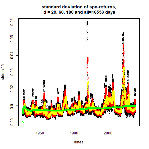
plot(dates,stddev20,main="standard deviation of spx-returns,\n d = 20, 60, 180 and all=16553 days")
points(dates,stddev60,col="red")
points(dates,stddev180,col="yellow")
points(dates,stddev_n,col="green")
# apparently: volatility is not constant
# normalized returns:
normret15 = dDayNormRet(15,ret)
normret60 = dDayNormRet(60,ret)
normret250 = dDayNormRet(250,ret)
normret_n = ret/stddev_n[n]

par(mfrow=c(2,2),oma=c(0,0,2,0))       #set up 2 time 2 plot array
                                       #that is, 4 pictures at once
hist(normret_n,breaks=150,xlim=c(-5,5),ylim=c(0,0.8),prob=TRUE,main="d = 16553 (all days)")
curve(dnorm(x),from=-5,to=5,add=TRUE,col="red")
hist(normret250,breaks=100,xlim=c(-5,5),ylim=c(0,0.8),prob=TRUE,main="d = 250")
curve(dnorm(x),from=-5,to=5,add=TRUE,col="red")
hist(normret60,breaks=50,xlim=c(-5,5),ylim=c(0,0.8),prob=TRUE,main="d = 60")
curve(dnorm(x),from=-5,to=5,add=TRUE,col="red")
hist(normret15,breaks=50,xlim=c(-5,5),ylim=c(0,0.8),prob=TRUE,main="d = 15")
curve(dnorm(x),from=-5,to=5,add=TRUE,col="red")
title(main="Histograms of d-Day Normalized S&P500 Returns",outer=TRUE)

# thus: if returns are normalized with more recent volatility
# data, then normalized returns are more Gaussian
-----------------------------------------------
# finally we take a single stock: #
# General Electric Company, since 1962: #
-----------------------------------------------
GE=read.table("C:/Users/Admin/Courses/FinancialStatistics/GE.txt",header=TRUE,sep=";")
head(GE)
tail(GE)
summary(GE) # no NA's
names(GE)
S = GE[,2]
dates = as.Date(GE$Date,format="%d-%m-%y")
dates # dates prior to 1969 have wrong year
datecorr = as.Date("1968-12-31") - as.Date("2068-12-31")
dates[1:1737] = dates[1:1737] + datecorr
dates
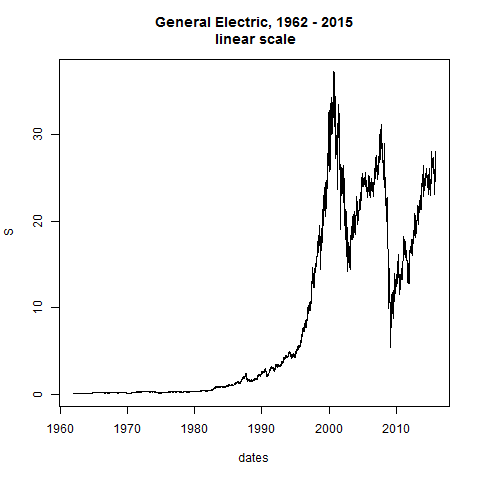
plot(dates,S,type="l",main="General Electric, 1962 - 2015\n linear scale")
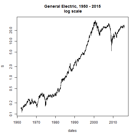
plot(dates,S,type="l",log="y",main="General Electric, 1950 - 2015\n log scale") # straight line would be constant exponential growth
n=length(S)
n
# we calculate the returns:
ret = rep(0,n)
for(i in 2:n)
{
ret[i] = (S[i]-S[i-1])/S[i-1]
}
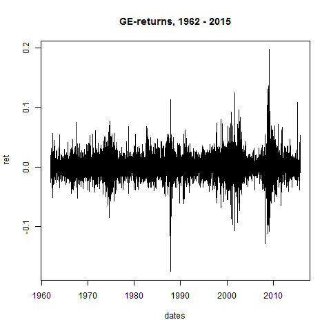
plot(dates,ret,type="l",main="GE-returns, 1962 - 2015")
# let's take a look at Stylized Fact 1:
mean20 = dDayMean(20,ret)
mean60 = dDayMean(60,ret)
mean180 = dDayMean(180,ret)
plot(dates,mean20,main="means of GE-returns, d = 20, 60 and 180 days")
points(dates,mean60,col="red")
points(dates,mean180,col="yellow")
# stddev's = daily volatilities:
stddev20 = dDayStdDev(20,ret)
stddev60 = dDayStdDev(60,ret)
stddev180 = dDayStdDev(180,ret)
stddev_n = dDayStdDev(n,ret)
plot(dates,stddev20,main="standard deviation of GE-returns,\n d = 20, 60, 180 and all=13540 days")
points(dates,stddev60,col="red")
points(dates,stddev180,col="yellow")
points(dates,stddev_n,col="green")
# apparently: volatility is not constant
# normalized returns:
normret15 = dDayNormRet(15,ret)
normret60 = dDayNormRet(60,ret)
normret250 = dDayNormRet(250,ret)
normret_n = ret/stddev_n[n]

par(mfrow=c(2,2),oma=c(0,0,2,0))       #set up 2 time 2 plot array
                                       #that is, 4 pictures at once
hist(normret_n,breaks=150,xlim=c(-5,5),ylim=c(0,0.8),prob=TRUE,main="d = 13540 (all days)")
curve(dnorm(x),from=-5,to=5,add=TRUE,col="red")
hist(normret250,breaks=100,xlim=c(-5,5),ylim=c(0,0.8),prob=TRUE,main="d = 250")
curve(dnorm(x),from=-5,to=5,add=TRUE,col="red")
hist(normret60,breaks=50,xlim=c(-5,5),ylim=c(0,0.8),prob=TRUE,main="d = 60")
curve(dnorm(x),from=-5,to=5,add=TRUE,col="red")
hist(normret15,breaks=50,xlim=c(-5,5),ylim=c(0,0.8),prob=TRUE,main="d = 15")
curve(dnorm(x),from=-5,to=5,add=TRUE,col="red")
title(main="Histograms of d-Day Normalized GE Returns",outer=TRUE)
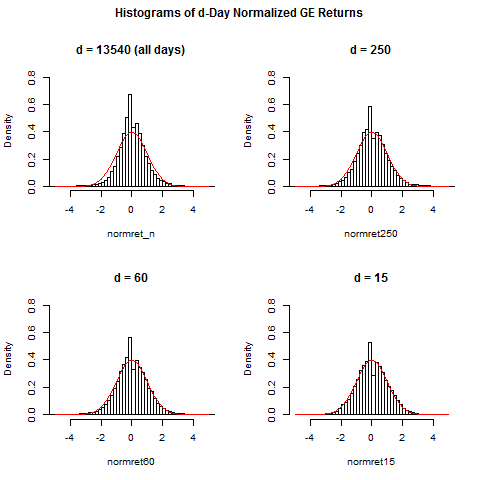
# thus: if returns are normalized with more recent volatility
# data, then normalized returns are more Gaussian


-------------------------------------------
#            Main   Conclusion:           #
-------------------------------------------

The normalized returns

normret_d(t_k) = ret(t_k) / stddev_d(t_{k-1})                (4)

may be approximated pretty well by a standard normal distri-
bution, if the time horizon d is chosen not too large: d=15
days or d=20 turned out to be quite reasonable choices.
Thus we can write

ret(t_k) / stddev_d(t_{k-1}) = phi_k                         (5)

with phi_k being a standard normal random number.
Equation (5) is equivalent to

S_k = S_{k-1} * [ 1 + stddev_d(t_{k-1}) * phi_k ]            (6)

Using the data which are known on day t_{k-1} and by drawing
a normally distributed random number, this equation gives us
a price for day t_k.

Now, is this a reasonable stochastic model? To this end we
will simulate a couple of paths with price dynamics given
by (6) in the next chapter and we will find that the model
actually cannot be used as exactly given by (6), but we have
to make some adjustments.