---------------------------------------------------
#                                                 #
#        Chapter 1: Compact Introduction          #
#                to the R-Software                #
#                                                 #
---------------------------------------------------

R-homepage:
https://cran.r-project.org/
The symbol # is the comment-symbol in R, all code 
after the #-symbol is ignored.


# There are 4 basic data types in R: vectors, 
# matrices, data frames and lists. Numbers are 
# vectors of lengths 1:

x = 7.7
y = 8.8
x+y

# There are basically 3 commands to generate vectors 
# in R: c(), seq() and rep()

v1 = c(2.22,-4.56,29)        # "c" for "concatenate"
v1
v2 = seq(from=10,to=30,by=2)
v2
v3 = seq(from=0,to=2*pi,length=100)
v3
plot(sin(v3))                # R always calculates element-wise

plot(sin(v3),type="l")
points(cos(v3))              # add points to an existing plot
lines(cos(v3),col="red")     # same as points, just of line-type

?plot                        # help-pages
v4 = rep(2,10)
v4
v5 = rep(c(77,33),4)
v5

# for vectors mit step size 1 or -1:

v6 = 1:10
v6
v7 = 10:30                   # increment is always 1 (or -1)
v7
v8 = 4:(-4)
v8
v8[1]
v8[2]
v8[7:9]
v8[7:11]

# many R-function automatically generate vectors as their 
# result:

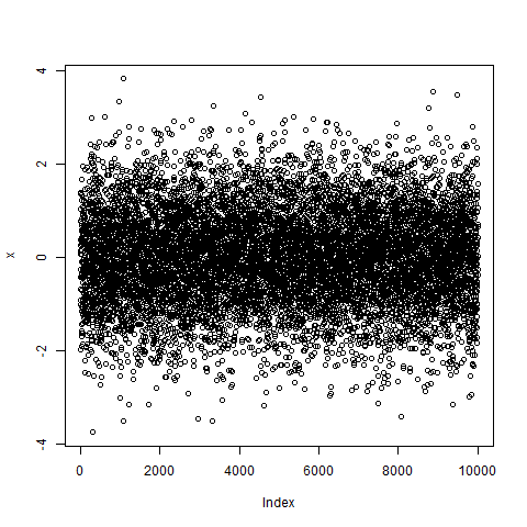
x = rnorm(10000)             # 10000 standard-normal random numbers
x
plot(x)

hist(x)

hist(x,prob=TRUE)
curve(dnorm(x),col="red",add=TRUE)

# R is pretty performant and offers lots of functionality
# for calculations with random numbers; for every 
# probability distribution dist there are the 4 functions 
#
# rdist    (generates random numbers)
# ddist    (the prob-density)
# pdist    (integral over the density)
# qdist    (inverse of pdist)


# Matrices:

x = 1:20
x
mat1 = matrix(x,nrow=4,ncol=5)
mat1
mat2 = matrix(x,nrow=5,ncol=4)
mat2
mat3 = matrix(x,nrow=5,ncol=4,byrow=TRUE)
mat3
mat3[2,4]
mat3[4:5,2]
mat3[4:5,2:3]

# R typically calculates element-wise:

x
x^2
x+0.33
1/x
mat3
mat3^2                       # this is not matrix-multiplication
mat3+0.77
1/mat3                       # this is not the inverse of a matrix

# Matrix-Multiplication:

mat4 = mat1 %*% mat2
mat4
det(mat4)                    # not invertible

v1=c(1,1,1)
v2=c(1,2,3)
v3=c(1,4,9)
mat5 = rbind(v1,v2,v3)       # "rowbind"
mat5
det(mat5)
mat5inv = solve(mat5)        # this is matrix-inverse
mat5inv
# check:
mat5 %*% mat5inv
zapsmall(mat5 %*% mat5inv)

# Eigenvalues und Eigenvectors of a Matrix:

n = 5                                # we repeat this for n=1000
x = rnorm(n*n)                       # n^2 random numbers
x
mat = matrix(x,nrow=n,ncol=n)        # nxn random matrix
mat
eigen(mat)
res = eigen(mat)
str(res)
names(res)

# the result of eigen(mat) is a list with 2 elements,  
# res[[1]]=res$values is of type vector and 
# res[[2]]=res$vectors is of type matrix.

# the main use of lists is to collect objects of different 
# data types into one single object. Often the return type 
# of R-functions is of type list, since these functions 
# provide various typs of information. For example, the 
# return type of the function lm() ("lm" for "linear model")
# which performs a linear regression, is a list with 13 
# elements.

res[[1]]
res$values
res[[2]]
res$vectors
n = 1000

# redo above, starting with code-line x = rnorm(n*n)  
# -> quite fast calculation of eigenvectors and values

plot(res$values)             # eigenvalues seem to be equally distributed
                             # in a cicle with radius, probably, sqrt(n)

# let's draw this circle and add to the plot of eigenvalues above:

phi = seq(from=0,to=2*pi,length=101)
r = sqrt(n)
z = r*exp(1i*phi)            # 1i is R-Syntax for complex i=sqrt(-1)
points(z,col="red",type="l")

# apparently R is able to compute with complex numbers:

z = 0.5 + sqrt(3)/2 *1i
z
Re(z)
Im(z)
abs(z)
arg(z)
Arg(z)                       # R is case-sensitive
Arg(z)/pi                    # 60 degrees


# Besides vectors, matrices and lists there is the data type 
# data frame. Typically, if some external data are imported 
# to R, they are stored in a data frame. 
# More on this in chapter2.