---------------------------------------------------
# #
# Chapter 4: The ARCH Time Series Model #
# #
---------------------------------------------------
In the last chapter we simulated the model
S(t_k) = S(t_{k-1}) * [ 1 + vol(t_{k-1})*phi_k ] (1)
with
vol^2(t_{k-1}) = stddev_d^2(t_{k-1})
= 1/d * [ret^2(t_{k-1})+...+ret^2(t_{k-d})] (2)
and we saw, that the volatility in that model converged
to zero, the simulated paths stayed constant after a
while. Apparently vol(t_{k-1}) = 0 and S(t_k) = const
is a solution of the equations (1,2) for arbitrary
random numbers phi_k. On the other hand, we saw that the
model
S(t_k) = S(t_{k-1}) * [ 1 + bsvol * phi_k ] (3)
with a constant Black-Scholes volatility bsvol does not
have this problem, the simulated paths looked quite
reasonable. However, the data analysis of chapter 2
clearly revealed that volatility is not constant and
a good model should take this into account. Therefore,
as a compromise between the models (1,2) and (3), we
make the Ansatz:
vol^2(t_{k-1}) = w0*bsvol^2 + w1*stddev_d(t_{k-1})^2 (4)
= w0 * bsvol^2 +
w1 * 1/d * [ret^2(t_{k-1})+...+ret^2(t_{k-d})]
with some positive weights w0 and w1 with
w0 + w1 = 1 .
The price dynamics (1) with vol-specification (4) is
called the ARCH-model or more precisely the ARCH(d)-
model, since the history of the past d days is taken
into account.
Before we simulate a couple of paths, let's make some
remarks:
Remark 1) The letters A, R, C and H stand for
AR = AutoRegressive, that means, future returns depend
on past returns, and:
CH = Conditional Heteroskedastic, that means, that the current,
instantaneous volatilities are time dependent.
There are conditional or instantaneous variances or
volatilities,
vol^2(t_{k-1}) = E[ ret^2(t_k) | t_{k-1} ]
-- the notation on the right meaning that until time
t_{k-1} everything is known and the expectation is
taken only over phi_k -- and unconditional variances
or volatilities,
volbar^2 = E[ ret^2(t_k) ]
where the expectation is taken over all phi_k,...,phi_1.
Heteroskedastic simply means: not constant, but time
dependent.
Remark 2) Instead of vol-specification (4) one could
make the more general Ansatz
vol^2(t_{k-1}) = alpha0 +
alpha1 * ret^2(t_{k-1}) + ... + alphad * ret^2(t_{k-d}) (5)
with some d+1 parameters alpha0,...,alphad. Typically
the specification (5) can be found in the books as the
definition of the ARCH(d)-model. However, if one really
wants to fit the model to actual time series data, one
would merely choose a parametrization (4), eventually
not necessasarily with equally weighted returns, but
with linearly or exponentially weighted returns. The
GARCH-model discussed in chapter 7 is basically an
ARCH(d)-model with exponentially weighted returns.
In addition, the parameters w0 and bsvol in (4) have an
immediate intuitive meaning: as we will see in later
chapters when we estimate the parameters with the
maximum likelihood method, bsvol is usually very close
to the standard deviation of the realized returns
calculated over the full length of the time series.
Thus, we don't have to estimate this parameter
actually, but can calculate it directly as sd(ret),
the standard deviation of the return series.
Remark 3) In 2003, Robert Engle from New York Uni-
versity (together with Clive Granger) was awarded
the Nobel Prize in Economics "for methods of analy-
zing economic time series with time-varying vola-
tility (ARCH)".
Now let's start and simply take a look at some
simulated paths. To this end, we modify our
pathNaivArch-function from the last chapter:
#
# Start R-Session:
#
pathArchd = function( N , bsvol , w0 , d )
{
S = rep(0,N)
ret = rep(0,N)
phi = rnorm(N)
S0 = 100
vol0 = bsvol # we put startvol to bsvol
vol = rep(vol0,N) # ARCH-vol
sumretd = 0
# the first step, k=1, is special:
S[1] = S0*(1+vol0*phi[1])
ret[1] = (S[1]-S0)/S0
vol[1] = sqrt( w0*bsvol^2 + (1-w0)*ret[1]^2 )
sumretd = sumretd + ret[1]^2
for(k in 2:N)
{
if(k<=d)
{
S[k] = S[k-1]*(1+vol[k-1]*phi[k])
ret[k] = (S[k]-S[k-1])/S[k-1]
sumretd = sumretd + ret[k]^2
vol[k] = sqrt( w0*bsvol^2 + (1-w0)*sumretd/k )
}
else
{
S[k] = S[k-1]*(1+vol[k-1]*phi[k])
ret[k] = (S[k]-S[k-1])/S[k-1]
sumretd = sumretd + ret[k]^2
sumretd = sumretd - ret[k-d]^2
vol[k] = sqrt( w0*bsvol^2 + (1-w0)*abs(sumretd)/d )
}
}#next k
par(mfrow=c(2,1))
plot(S,type="l",ylim=c(0,250))
plot(ret,type="l",ylim=c(-0.08,0.08))
result = list(S,ret)
names(result) = c("S","ret")
return(result)
}
#
# let's check:
#
# this should be Black-Scholes:
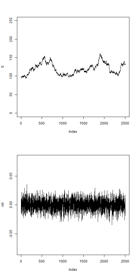
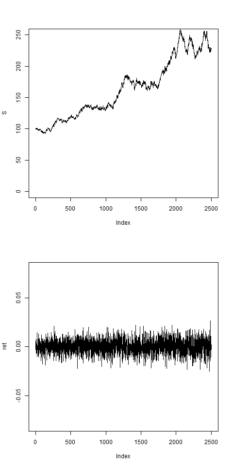
res = pathArchd( N=2500 , bsvol=0.01 , w0=1 , d=15 )
# returns are uniformly distributed:
# this is with variable vol:
res = pathArchd( N=2500 , bsvol=0.01 , w0=0.5 , d=15 )
# vol looks still quite uniform:
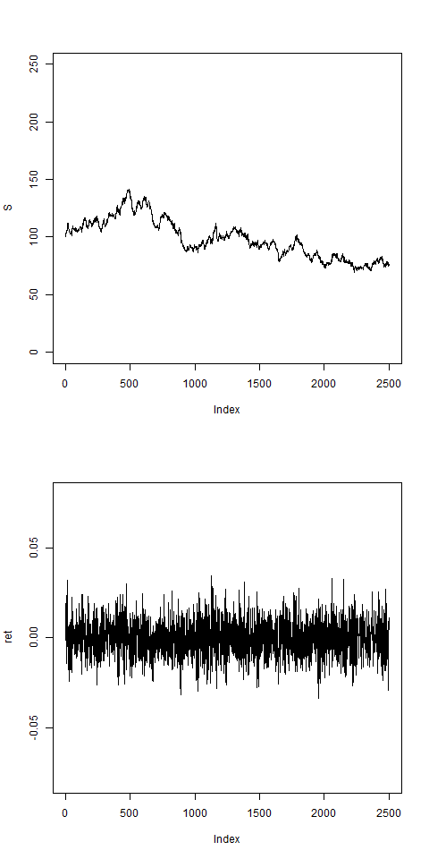
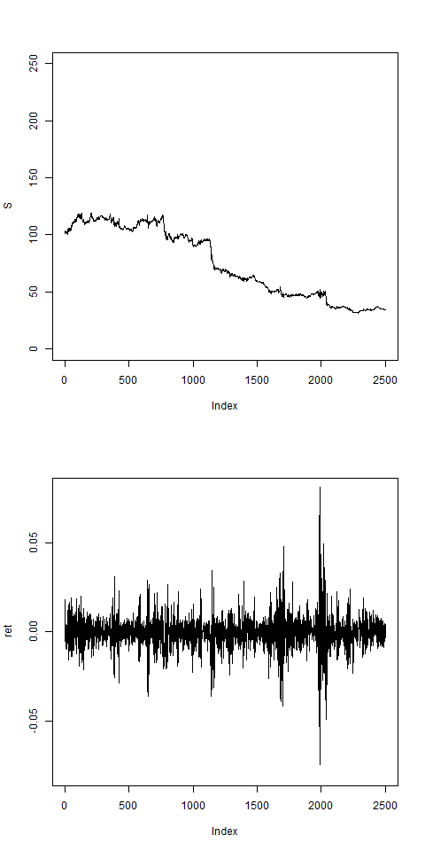
res = pathArchd( N=2500 , bsvol=0.01 , w0=0.1 , d=15 )
# this shows vol clustering:
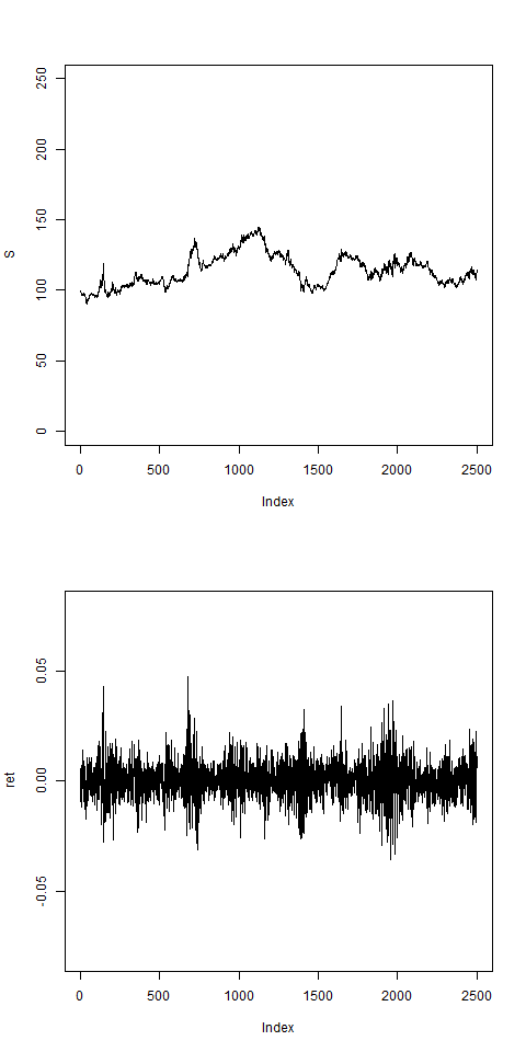
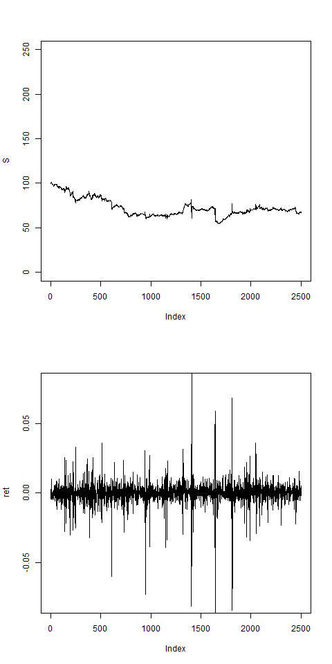
res = pathArchd( N=2500 , bsvol=0.01 , w0=0.1 , d=10 )
# this shows vol clustering:
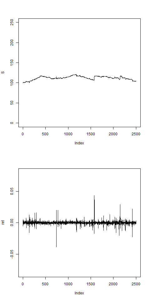
res = pathArchd( N=2500 , bsvol=0.01 , w0=0.1 , d=250 )
# for large d, returns become more uniform:
res = pathArchd( N=2500 , bsvol=0.01 , w0=0.1 , d=5 )
# this shows vol clustering:
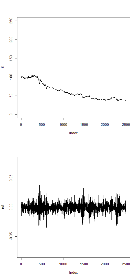
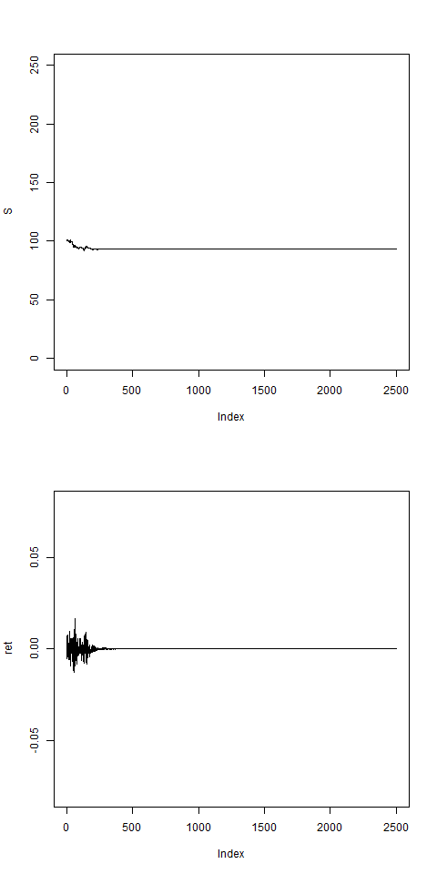
res = pathArchd( N=2500 , bsvol=0.01 ,w0=0.1 , d=1 )
res = pathArchd( N=2500 , bsvol=0.01 ,w0=0.01 , d=1 )
res = pathArchd( N=2500 , bsvol=0.01 ,w0=0    , d=1 )
# w0 > 0 necessary to stabilizes the model:
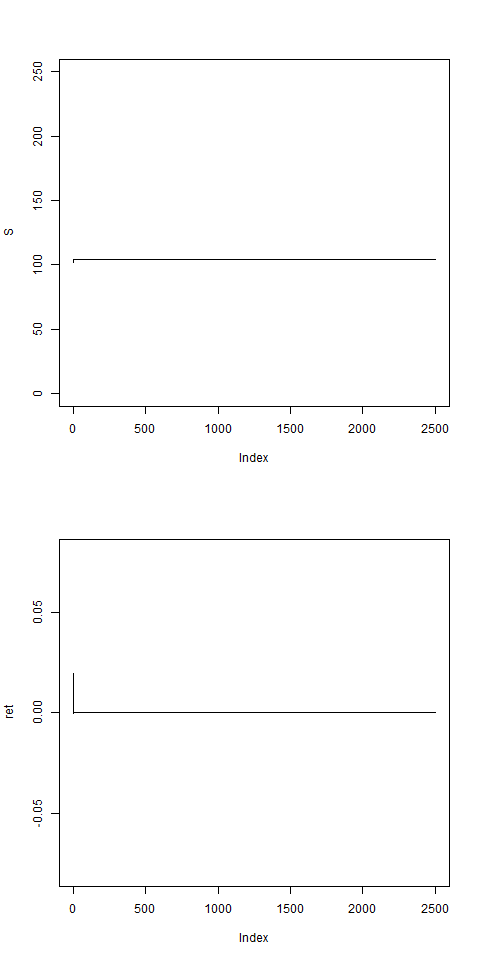
res = pathArchd( N=2500 , bsvol=0.01 ,w0=0    , d=15 )
# w0 > 0 necessary to stabilizes the model:
# a realistic set of parameters:
res = pathArchd( N=2500 , bsvol=0.015 ,w0=0.15, d=15 )
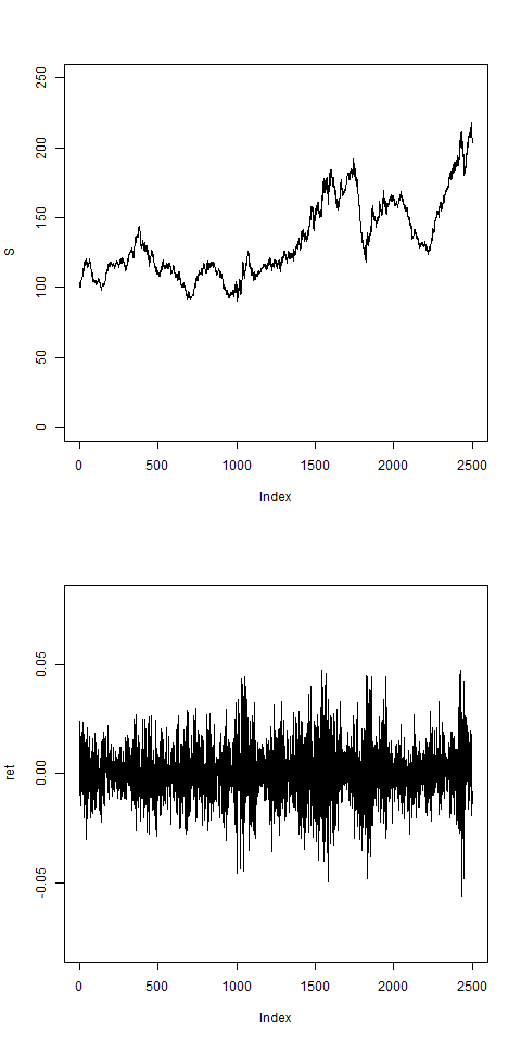
This looks not unreasonable. Now we can start to fit
the model to actual time series data. This we will do
in the next chapter with the maximum likelihood method.