---------------------------------------------------
# #
# Chapter 6: Maximum Likelihood Estimation #
# of the ARCH(d)-Model #
# #
---------------------------------------------------
In the last chapter we familiarized ourselves with the
maximum likelihood method and we derived the following
expression for the log-likelihood function (we discarded
a constant involving logarithms of 2*pi's):
log(L) = (1)
- sum_{k=1}^N { log[vol(t_{k-1})] + 1/2 * y_k^2 / vol^2(t_{k-1}) }
The y_k are given by the realized returns of the actual
time series data,
y_k = ret(t_k) = [ S(t_k)-S(t_{k-1}) ] / S(t_{k-1}) (2)
and the exact form of the volatility vol(t_k) depends
on the model under consideration. For the ARCH(1)-model,
it is given by
vol^2(t_{k-1}) = w0*bsvol^2 + (1-w0)*ret^2(t_{k-1}) (3)
with w0 and bsvol being the model parameters. For the
DAX time series, we found
DAX: w0 = 0.7 und bsvol = 1.4% (4)
by maximizing the ARCH(1) log-likelihood function. The
parameter bsvol of 1.4% turned out to be very close to
the standard deviation sd(ret) of the returns taken over
the whole time series length, sd(ret) = 1.39%.
The more realistic ARCH(d)-model which is to be estimated
in this chapter has the following vol-specification:
vol^2(t_{k-1}) =
w0*bsvol^2 + (1-w0)*[ret^2(t_{k-1})+...+ret^2(t_{k-d})] / d (5)
with ARCH(d) model parameters w0, bsvol and the time
horizon d. The maximization of the likelihood function
again has to be done numerically and to this end we
start an R-session:
# Start R-Session:
#
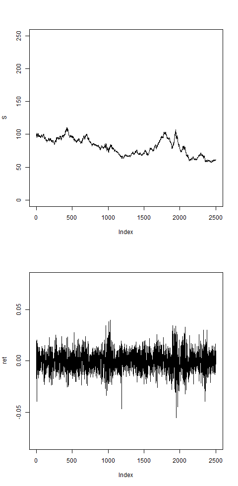
# before we fit to DAX-data, we check on an artificially
# generated ARCH(d) return set: let's use the pathArchd
# function from the last chapter to generate these arti-
# ficial return data:
pathArchd = function( N , bsvol , w0 , d )
{
S = rep(0,N)
ret = rep(0,N)
phi = rnorm(N)
S0 = 100
vol0 = bsvol # we put startvol to bsvol
vol = rep(vol0,N) # ARCH-vol
sumretd = 0
# the first step, k=1, is special:
S[1] = S0*(1+vol0*phi[1])
ret[1] = (S[1]-S0)/S0
vol[1] = sqrt( w0*bsvol^2 + (1-w0)*ret[1]^2 )
sumretd = sumretd + ret[1]^2
for(k in 2:N)
{
if(k<=d)
{
S[k] = S[k-1]*(1+vol[k-1]*phi[k])
ret[k] = (S[k]-S[k-1])/S[k-1]
sumretd = sumretd + ret[k]^2
vol[k] = sqrt( w0*bsvol^2 + (1-w0)*sumretd/k )
}
else
{
S[k] = S[k-1]*(1+vol[k-1]*phi[k])
ret[k] = (S[k]-S[k-1])/S[k-1]
sumretd = sumretd + ret[k]^2
sumretd = sumretd - ret[k-d]^2
vol[k] = sqrt( w0*bsvol^2 + (1-w0)*abs(sumretd)/d )
}
}#next k
par(mfrow=c(2,1))
plot(S,type="l",ylim=c(0,250))
plot(ret,type="l",ylim=c(-0.08,0.08))
result = list(S,ret)
names(result) = c("S","ret")
return(result)
}
# we generate an artificial ARCH(d) return set where we
# know the actual model parameters ( bsvol , w0 , d ):
# let's set a seed for the random numbers to make this
# reproducible:
set.seed(234)
N = 2500
bsvol = 0.01
w0 = 0.3
d = 20
res = pathArchd( N , bsvol , w0 , d )
ret = res$ret
summary(ret)


# we have to calculate the log-Likelihood function:
#
# use 'vectorized' calculation logic of R to make the code
# a bit more performant -> code looks a bit less intuitive:


logL = function( bsvol , w0 , d )
{
  w1 = 1 - w0
  n = length(ret)

  cumsum_retsquared = cumsum(ret^2)

  # remove last d elements:
  cumsum_retsquared_shifted = cumsum_retsquared[-((n-d+1):n)]

  # fill in d zeros at the first d places:
  cumsum_retsquared_shifted = c(rep(0,d),cumsum_retsquared_shifted)

  sum_dretsquared = cumsum_retsquared - cumsum_retsquared_shifted

  # now we have to divide this sum by d, but the first d elements
  # are special:
  divisor1 = 1:d
  divisor2 = rep(d,n-d)
  divisor = c(divisor1,divisor2)

  sum_dretsquared = sum_dretsquared/divisor

  # now we can calculate ARCH(d)-vol:
  vol = sqrt( w0*bsvol^2 + w1*sum_dretsquared )

  # shift vol-vector by 1 element ( there is a vol(t_{k-1}) in
  # the likelihood-function, not a vol(t_k) )
  vol = vol[-n]                           # remove last one
  vol = c(sqrt(w0*bsvol^2),vol)           # add a new first one

  # the actual calculation:
  terms = log(vol) + 1/2*ret^2/vol^2
  result = -sum(terms)

  return(result)
}


# let's check:
logL( bsvol=0.01, w0=0.3, d=20 )          # alright, some number

# let's look for the maximum:
# first, we fix bsvol to its natural value:
bsvol = sd(ret)
bsvol

# we make a contour-plot in the (w0,d)-plane:

w0 = seq(from=0.05,to=0.95,by=0.05)
dd = 1:40
nw = length(w0)
nd = length(dd)

# matrix z = logL for contour-plot:
z = matrix( 0 , nrow=nd , ncol=nw )
for(i in 1:nd)
{
  for(j in 1:nw )
  {
    z[i,j] = logL( bsvol , w0[j] , dd[i] )
  }
}# still very fast evaluation of logL!

# let's look at the result:
contour( dd , w0 , z , nlevels = 50 )
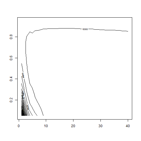
contour( dd , w0 , z , nlevels = 50 , zlim=c(10000,11000) )
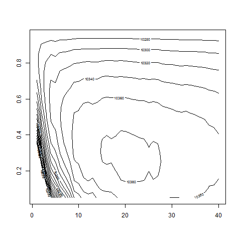
contour( dd , w0 , z , nlevels = 100 , zlim=c(10200,10600) )

# we recover correct parameter values:
# d around 20 and w0 around 0.3;
# differences between d = 15, 20 and 25 not that big,
# depending on the particular realization of random numbers;
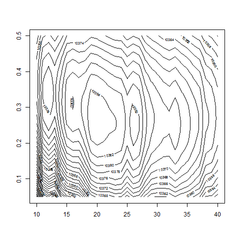
# d below 8 clearly less favorable -> redo calculation for
# dd = 10:40 and w0 < 0.5 (-> resolution on pictures more nice)
w0 = seq(from=0.05,to=0.5,by=0.01)
dd = 10:40
nw = length(w0)
nd = length(dd)
z = matrix( 0 , nrow=nd , ncol=nw )
for(i in 1:nd)
{
for(j in 1:nw )
{
z[i,j] = logL( bsvol , w0[j] , dd[i] )
}
}
contour( dd , w0 , z , nlevels = 150 , zlim=c(10200,10600) )
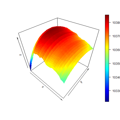
# some more pictures:
image( dd , w0 , z )
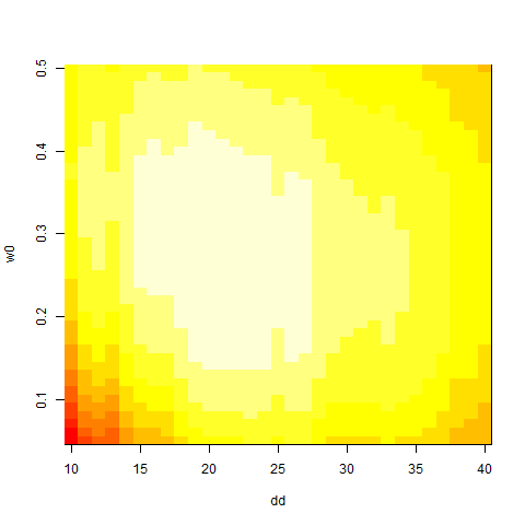
persp( dd , w0 , z )
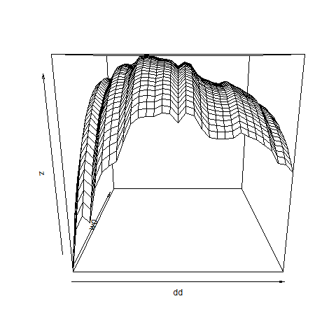
require(plot3D)
persp3D( dd , w0 , z )
# let's fix d=20 and check that bsvol=sd(ret) corresponds
# to the maximum:

bsvol = seq(from=0.1/100,to=4/100,by=0.1/100)
nbs = length(bsvol)
z = matrix( 0 , nrow=nbs , ncol=nw )
for(i in 1:nbs)
{
  for(j in 1:nw )
  {
    z[i,j]=logL( bsvol[i] , w0[j] , d=20 )
  }
}
contour( bsvol , w0 , z , nlevels = 50 )
contour( bsvol , w0 , z , nlevels = 80 , zlim=c(10000,10500) )
# -> looks all good.
#
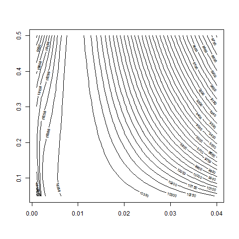
# finally, let's fix w0 and vary bsvol and d:
#
bsvol = seq(from=0.1/100,to=2/100,by=0.05/100)
nbs = length(bsvol)
dd = 10:40
nd = length(dd)
z = matrix( 0 , nrow=nd , ncol=nbs )
for(i in 1:nd)
{
for(j in 1:nbs )
{
z[i,j]=logL( bsvol[j] , w0=0.3 , d=dd[i] )
}
}
contour( dd , bsvol , z , nlevels = 50 )

-----------------------------------------
# ARCH(d)-Fit to DAX-Data: #
-----------------------------------------
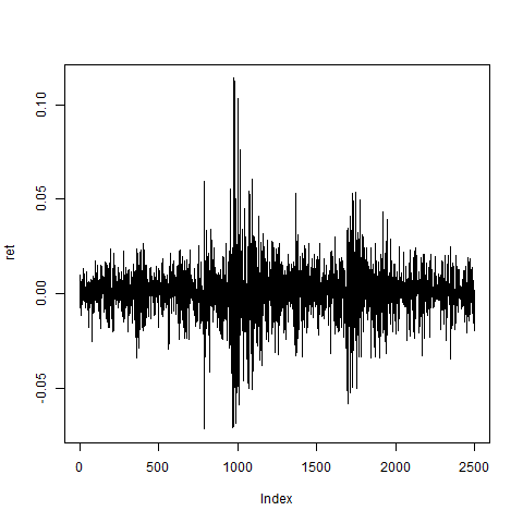
dax = read.table("C:/Users/Admin/Courses/FinancialStatistics/DAX.txt",header=TRUE,sep=";")
dax = na.omit(dax)
summary(dax)
rm(ret)
S = dax$index
n=length(S)
ret = rep(0,n)
for(i in 2:n)
{
ret[i] = (S[i]-S[i-1])/S[i-1]
}
plot(ret,type="l")
w0 = seq(from=0.05,to=0.95,by=0.05)
dd = 1:40
bsvol = sd(ret)
bsvol
nw = length(w0)
nd = length(dd)
z = matrix( 0 , nrow=nd , ncol=nw )
for(i in 1:nd)
{
  for(j in 1:nw )
  {
    z[i,j] = logL( bsvol , w0[j] , dd[i] )
  }
}

# let's look at the result:
contour( dd , w0 , z , nlevels = 50 )
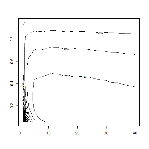
contour( dd , w0 , z , nlevels = 50 , zlim=c(9500,10500) )

# apparently w0 less than 0.4 and d between 8 and 28:

w0 = seq(from=0.01,to=0.4,by=0.01)
dd = 8:28
bsvol = sd(ret)
#
# reevaluate z with the code above
#
contour( dd , w0 , z , nlevels = 50 , zlim=c(9500,10500) )
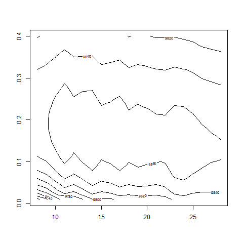
contour( dd , w0 , z , nlevels = 100 , zlim=c(9800,10000) )
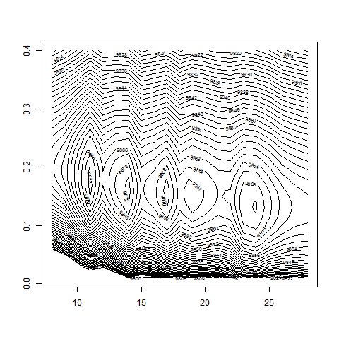
# -> d = 14 and w0 around 0.15:
max(z) # 9873.06
logL( bsvol=sd(ret) , w0=0.15 , d=14 ) # 9872.65
# some more pictures:
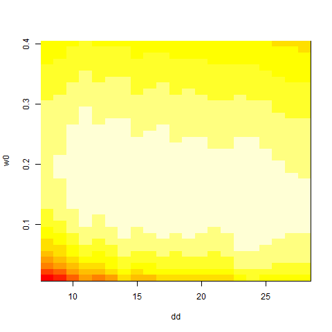
image( dd , w0 , z )
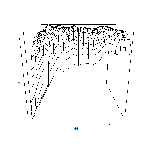
persp( dd , w0 , z )
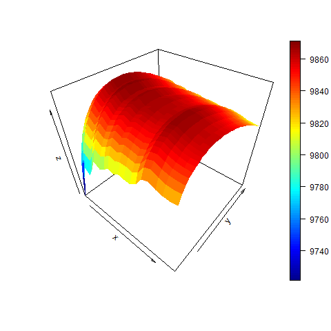
persp3D( dd , w0 , z )
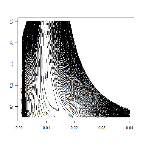
# finally we check for bsvol:
w0 = seq(from=0.01,to=0.4,by=0.01)
bsvol = seq(from=0.1/100,to=4/100,by=0.1/100)
nbs = length(bsvol)
z = matrix( 0 , nrow=nbs , ncol=nw )
for(i in 1:nbs)
{
  for(j in 1:nw )
  {
    z[i,j]=logL( bsvol[i] , w0[j] , d=14 )
  }
}
contour( bsvol , w0 , z , nlevels = 50)
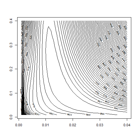
contour( bsvol , w0 , z , nlevels = 80 , zlim=c(9800,10000))
max(z) # 9872.76
logL( bsvol=sd(ret) , w0=0.15 , d=14 ) # 9872.65
# -> Maximum at w0=15%, bsvol=sd(ret)=1.39%, d=14.
-----------------------------------------
# ARCH(d)-Fit to SPX-Data: #
-----------------------------------------
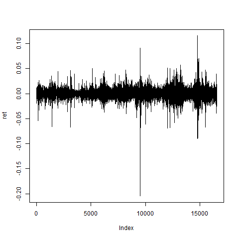
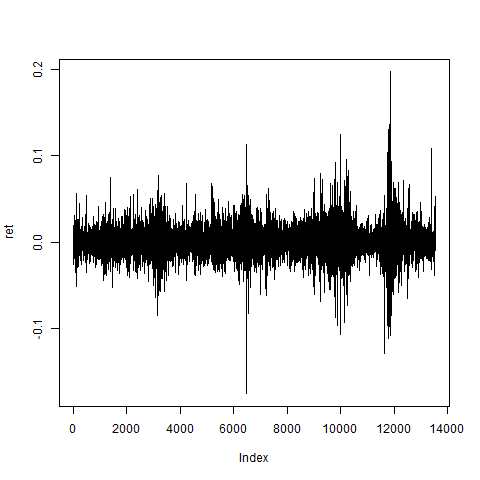
# load SPX.txt data and generate return vector ret:
spx = read.table("C:/Users/Admin/Courses/FinancialStatistics/spx.txt",header=TRUE,sep=";")
head(spx)
summary(spx) # no NA's
S = spx[,2]
n = length(S)
ret = rep(0,n)
for(i in 2:n)
{
ret[i] = (S[i]-S[i-1])/S[i-1]
}
plot(ret,type="l") # returns look ok
# compute spx-logL and make setup for contour-plot:
# first, we fix bsvol to its natural value:
bsvol = sd(ret)
bsvol
# we make a contour-plot in the (w0,d)-plane:
w0 = seq( from=0.05 , to=0.95 , by=0.05 )
dd = 1:40
nw = length(w0)
nd = length(dd)
z = matrix( 0 , nrow=nd , ncol=nw )
for(i in 1:nd)
{
for(j in 1:nw )
{
z[i,j] = logL( bsvol , w0[j] , dd[i] )
}
}
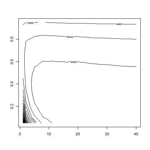
contour( dd , w0 , z , nlevels = 50 )
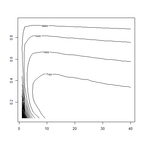
contour( dd , w0 , z , nlevels = 80 , zlim=c(70000,72000) )
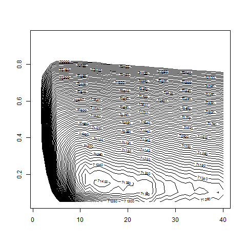
# apparently w0 less than 0.3 and d between 8 and 28:
w0 = seq( from=0.01 , to= 0.3 , by=0.005 )
dd = 8:28
#
# reevaluate z = logL with the code above
#
contour( dd , w0 , z , nlevels = 100 , zlim=c(70000,72000) )
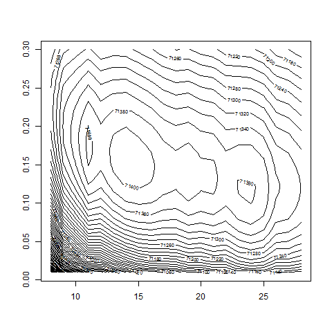
contour( dd , w0 , z , nlevels = 200 , zlim=c(71000,72000) )
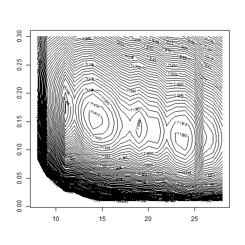
# -> d = 14  and w0 around 0.15
max(z)                                         # 71413.99
logL( bsvol=sd(ret) , w0=0.15 , d=14 )         # 71413.54

# some more pictures:
persp( dd , w0 , z )
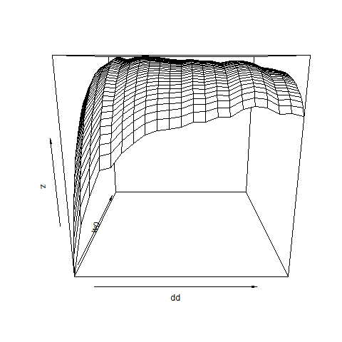
persp3D( dd , w0 , z )
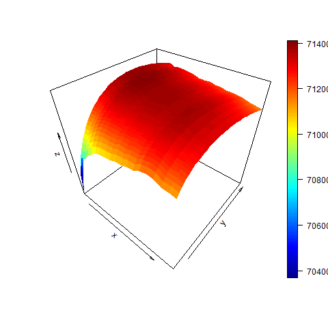
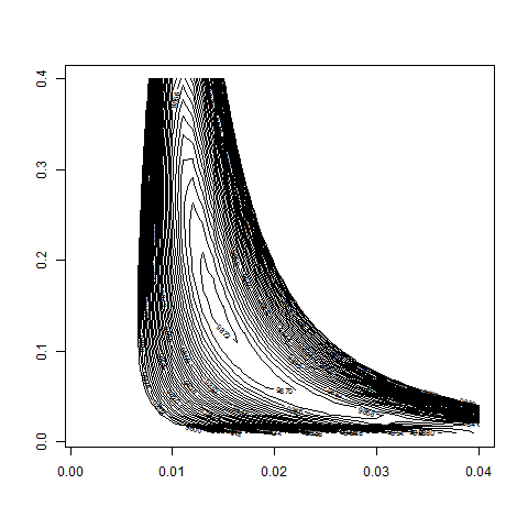
# finally we check for bsvol:
w0 = seq( from=0.01 , to=0.3 , by=0.005 )
bsvol = seq( from=0.1/100 , to=2/100 , by=0.05/100 )
nbs = length(bsvol)
nw = length(w0)
z = matrix( 0 , nrow=nbs , ncol=nw )
for(i in 1:nbs)
{
  for(j in 1:nw )
  {
    z[i,j]=logL( bsvol[i] , w0[j] , d=14 )
  }
}
contour( bsvol , w0 , z , nlevels = 100 , zlim=c(70000,72000) )

contour( bsvol , w0 , z , nlevels = 200 , zlim=c(71000,72000) )
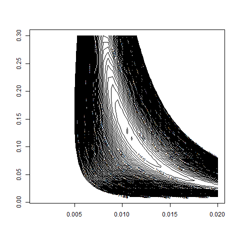
# thus: Maximum at approximately
logL( bsvol=sd(ret) , w0=0.15 , d=14 )         # 71413.54
max(z)                                         # okay..
sd(ret)


-----------------------------------------
#       ARCH(d)-Fit to GE-Data:         #
-----------------------------------------

# load GE.txt data and generate return vector ret:
ge = read.table("C:/Users/Admin/Courses/FinancialStatistics/GE.txt",header=TRUE,sep=";")
head(ge)
summary(ge)     # no NA's
S = ge[,2]
n = length(S)
ret = rep(0,n)
for(i in 2:n)
{
  ret[i] = (S[i]-S[i-1])/S[i-1]
}
plot(ret,type="l")   # returns look ok
# compute GE-logL and make setup for contour-plot:
# first, we fix bsvol to its natural value:
bsvol = sd(ret)
bsvol
# we make a contour-plot in the (w0,d)-plane:
w0 = seq( from=0.05 , to=0.95 , by=0.05 )
dd = 1:40
nw = length(w0)
nd = length(dd)
z = matrix( 0 , nrow=nd , ncol=nw )
for(i in 1:nd)
{
  for(j in 1:nw )
  {
    z[i,j] = logL( bsvol , w0[j] , dd[i] )
  }
}
contour( dd , w0 , z , nlevels = 50 )
contour( dd , w0 , z , nlevels = 70 , zlim=c(50000,51000) )

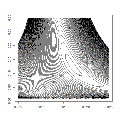
# apparently w0 less than 0.3 and d between 10 and 50:
w0 = seq( from=0.01 , to= 0.3 , by=0.005 )
dd = 10:50
#
# reevaluate z = logL with the code above
#
contour( dd , w0 , z , nlevels = 70 , zlim=c(50000,51000) )
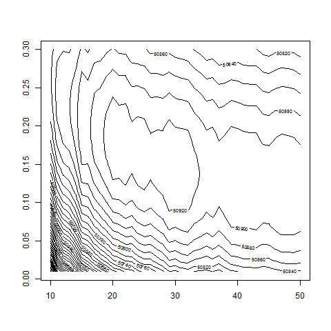
contour( dd , w0 , z , nlevels = 100 , zlim=c(50500,51000) )
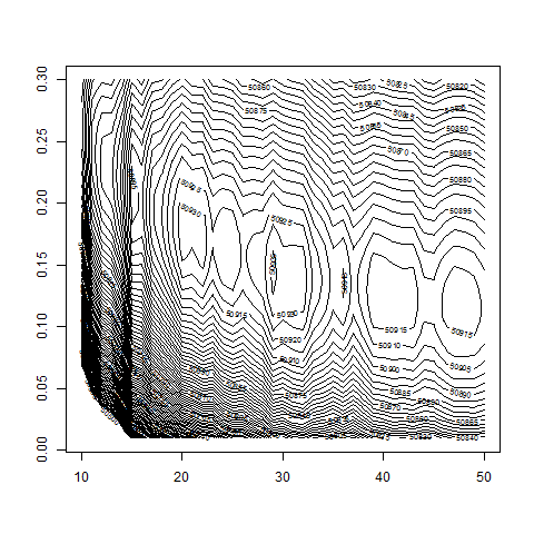
# -> d = 29 and w0 around 0.15
max(z) # 50936.45
logL( bsvol=sd(ret) , w0=0.15 , d=29 ) # 50936.28
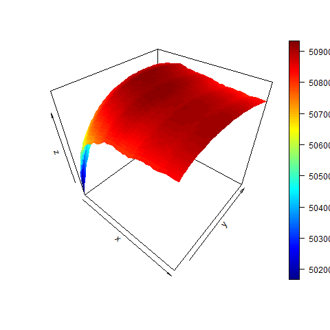
# some more pictures:
persp( dd , w0 , z )
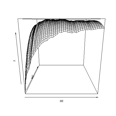
persp3D( dd , w0 , z )
# finally we check for bsvol:
w0 = seq( from=0.01 , to=0.3 , by=0.005 )
bsvol = seq( from=0.5/100 , to=2.5/100 , by=0.05/100 )
nbs = length(bsvol)
nw = length(w0)
z = matrix( 0 , nrow=nbs , ncol=nw )
for(i in 1:nbs)
{
  for(j in 1:nw )
  {
    z[i,j]=logL( bsvol[i] , w0[j] , d=29 )
  }
}
contour( bsvol , w0 , z , nlevels = 50)
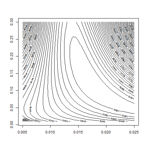
contour( bsvol , w0 , z , nlevels = 100 , zlim=c(50500,51000) )
# thus: Maximum at approximately
logL( bsvol=sd(ret) , w0=0.15 , d=29 )        # 50936.28
max(z)                                        # 50936.61
sd(ret)   # 1.62%