----------------------------------------------------
#                                                  #
#    Chapter 5: Maximum Likelihood Estimation      #
#                of the ARCH(1)-Model              #
#                                                  #
----------------------------------------------------



In the last chapter we defined the ARCH(d)-model and 
we simulated a couple of paths for various choices 
of model paramters. We saw that, depending on the 
choice of these model parameters, the model is already 
able to generate quite a variety of different price 
dynamics.

Now the question arises how we can determine which of 
these price dynamics, that is, which choice of model 
parameters, are the best for a given time series. 
In this chapter we will answer this question for the 
ARCH(1)-model. The logic for the ARCH(d)-model is 
completely analog and will be considered in the next 
chapter.


The ARCH(1)-Model is given by 

S(t_k) = S(t_{k-1}) * [ 1 + vol(t_{k-1})*phi_k ]                  (1)

with volatility specification 

vol^2(t_{k-1}) = w0*bsvol^2 + w1*ret^2(t_{k-1})                   (2)

with weights  w0+w1=1  and a constant Black-Scholes 
volatility bsvol. For  w0=1, w1=0  the model reduces 
to the time discrete Black-Scholes model (with zero 
drift).  

Let's fit this model to the DAX time series. That is, 
we would like to determine the parameters w0 (then 
w1=1-w0 is also fixed) and bsvol, such that the 
corresponding price dynamics fits `best' to the given 
time series data. The meaning of `best' of course 
has to be formulated in some precise mathematical way.

To this end we rewrite (1) as 

ret(t_k) = vol(t_{k-1}) * phi_k                                   (3)

and recall, that phi_k is a standard normal-distributed 
random number. Thus, if we are at time t_{k-1}, then 
the probability that the next return ret(t_k) will 
realize in the intervall [y_k,y_k+dy_k], is given by


Prob[ ret(t_k) in [y_k,y_k+dy_k] | t_{k-1} ]                      (4)

 = 1/sqrt{2pi} 1/vol(t_{k-1}) * exp( -1/2*y_k^2/vol^2(t_{k-1}) ) dy_k


Thus, the probability that all returns have values in 
some intervalls [y_k,y_k+dy_k], for all k=1,2,...,N, 
is given by the product of the probabilities in (4), 


Prob[ DAX-ret in [y_k,y_k+dy_k] for all k ] 

  = prod_{k=1}^N 1/sqrt{2pi} 1/vol(t_{k-1}) *                     (5)

    prod_{k=1}^N exp( -1/2*y_k^2/vol^2(t_{k-1}) ) dy_k


Now, if we substitute the ARCH(1) vol-specification given
by (2) above, 

vol^2(t_{k-1}) = w0*bsvol^2 + w1*y_{k-1}^2                        (2)

on the right hand side of (5), then the probability in (5),

Prob[ DAX-ret in [y_k,y_k+dy_k] for all k ] 

can be considered as a function of the model parameters 
bsvol and w0 exclusively, since the y_k are actually to be 
substituted by the actual realized returns of the last 10 
years. To make this more explicit, that we actually consider 
this probability as a function of the model parameters 
bsvol and w0, we introduce a new letter L (for "Likelihood") 
and write


Prob[ DAX-ret in [y_k,y_k+dy_k] for all k ] 

  =  L( w0 , bsvol )                                              (6)

  =  L( w0 , bsvol | y_k=ret(t_k) )                                   


where the notation in the last line of (6) should just be a 
reminder that the y_k are given data, namely the returns 
which have realized. This L is then called the likelihood 
function and a standard procedure in statistics is simply to 
estimate model parameters by maximizing this likelihood func-
tion. Accordingly, this method is called "Maximum Likelihood 
Estimation".



Since we have about N=2500 returns in a time series of 10 
years, L is given by a product of N=2500 factors. Thus, we 
should expect that L behaves like

  L ~ exp( +N*something )  or   L ~ exp( -N*something )           (7)

which is either extremely large or extremely small. To avoid 
numerical issues, it is therefore common to consider the 
logarithm log(L) of the likelihood function. Apparently, 
maximizing L is equivalent of maximizing log(L), so the logic 
stays the same, but for log(L) we can expect a behaviour of 

  log(L) ~  +N*something   or   log(L) ~  -N*something            (8)

which is much more tractable than the expressions in (7). 
Thus we consider

log(L) = sum_{k=1}^N { log[1/vol(t_{k-1})] -                      (9)

                       1/2 * y_k^2 / vol^2(t_{k-1}) } 
         + const

where the constant 

const = N*log[1/sqrt{2pi}] + sum_{k=1}^N log[dy_k]               (10)

does not depend on the model paramters w0 and bsvol. Since 
we maximize with respect to model parameters, we therefore 
can ignore the constant (10) and end up with the problem of 
maximizing the function  


log(tilde L) = log(tilde L)( bsvol , w0 )                        (11)

= - sum_{k=1}^N { log[vol(t_{k-1})] + 1/2 * y_k^2 / vol^2(t_{k-1}) }        

with  y_k = ret(t_k)  and

vol^2(t_{k-1}) = w0*bsvol^2 + (1-w0)*ret^2(t_{k-1})               (2)


This maximization problem has no longer an analytic closed 
form solution and one has to resort to some kind of numerical 
method. This is actually a typical situation in Maximum Likeli-
hood Estimation: the maximum cannot be found in analytic closed 
form, but has to be computed numerically. 

We make an R-implementation to perform this task:



# Start R-Session: 
#
# before we fit to DAX-data, we check on an artificially 
# generated ARCH(1) return set: let's use the pathArchd 
# function from the last chapter with d=1 to generate these 
# artificial return data:

# to make this reproducible, we fix a seed for 
# the random number generator:
set.seed(456)

pathArchd = function( N , bsvol , w0 , d )
{
  S = rep(0,N)
  ret = rep(0,N)
  phi = rnorm(N)
  S0 = 100
  vol0 = bsvol            # we put startvol to bsvol
  vol = rep(vol0,N)       # ARCH-vol

  sumretd = 0

  # the first step, k=1, is special:
  S[1] = S0*(1+vol0*phi[1])
  ret[1] = (S[1]-S0)/S0
  vol[1] = sqrt( w0*bsvol^2 + (1-w0)*ret[1]^2 )
  sumretd = sumretd + ret[1]^2

  for(k in 2:N)
  {
    if(k<=d)
    {
      S[k] = S[k-1]*(1+vol[k-1]*phi[k])
      ret[k] = (S[k]-S[k-1])/S[k-1]
      sumretd = sumretd + ret[k]^2
      vol[k] = sqrt( w0*bsvol^2 + (1-w0)*sumretd/k )
    }
    else
    {
      S[k] = S[k-1]*(1+vol[k-1]*phi[k])
      ret[k] = (S[k]-S[k-1])/S[k-1]
      sumretd = sumretd + ret[k]^2
      sumretd = sumretd - ret[k-d]^2
      vol[k] = sqrt( w0*bsvol^2 + (1-w0)*abs(sumretd)/d )
    }
  }#next k
  
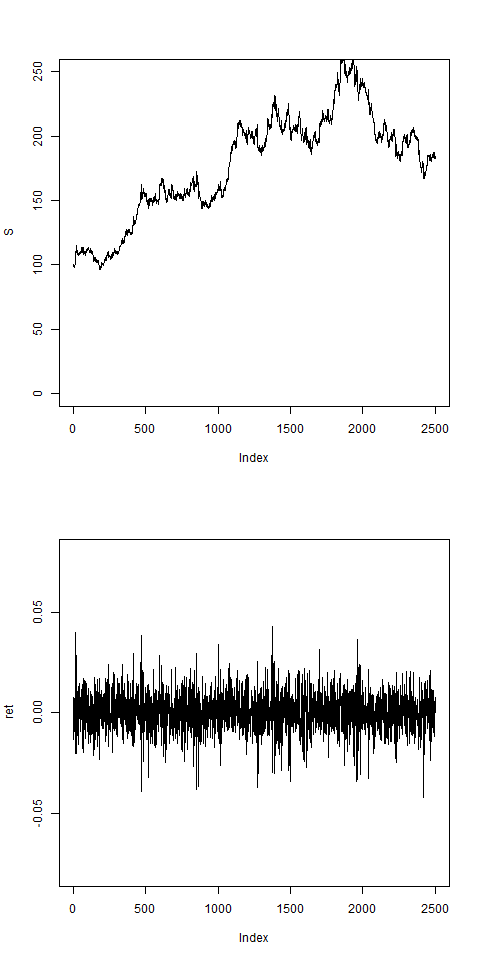
  par(mfrow=c(2,1))
  plot(S,type="l",ylim=c(0,250))
  plot(ret,type="l",ylim=c(-0.08,0.08))

  result = list(S,ret)
  names(result) = c("S","ret")
  return(result)
}

N = 2500
bsvol = 0.01
w0 = 0.5
res = pathArchd( N , bsvol , w0 , d=1 )
ret=res$ret
summary(ret)

# artificially generated price path 
# and return set:

# for this return set ret we now want to calculate the 
# log-likelihood function and a maximization should 
# result in model parameters around bsvol = 1% = 0.01 
# and w0 = 0.5:
#
# we calculate the log-Likelihood function:

logL = function( bsvol , w0 )
{
  w1 = 1 - w0
  vol = sqrt(w0*bsvol^2+w1*ret^2)     # we can use the vector ret, although we
                                      # did not pass it through the arguments
  # shift vol by 1 element:
  n = length(ret)
  vol = vol[-n]                       # remove last one
  vol = c(sqrt(w0*bsvol^2),vol)       # add a new first one
  terms = log(vol) + 1/2*ret^2/vol^2
  result = -sum(terms)
  return(result)
}


# let's check:
logL( bsvol=0.01 , w0=0.5 )           # ok, we get some number


# since we have only 2 variables, we can look for the maximum 
# by making a contour-plot. To become familiar with the 
# contour()-function, let's first consider an example:


#-----------------------------------------------------
# START Example: Contour-Plot:
#
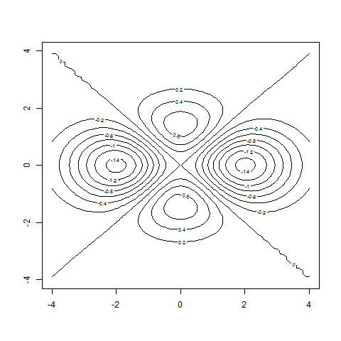
# function of 2 variables to be plotted:

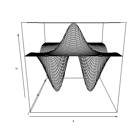
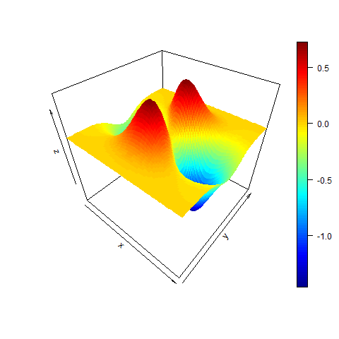
testf = function(x,y)
{
  result = (-x^2+y^2)*exp(-0.25*x^2-0.5*y^2)
  return(result)
}

# the contour()-command has syntax 
# contour(  vector ,  vector , matrix ) = 
# contour( x-Achse , y-Achse , f(x,y) )


x = seq(from=-4,to=4,by=0.1)
y = x

# matrix with testf(x,y)-values:
z = outer( x , y , FUN = testf )     # this works only if the function testf can 
                                     # accept vectors as input variables

# and now the level curves:
contour( x , y , z )

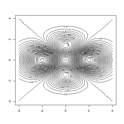
contour( x , y , z , nlevels=50 )    # more refined

# instead of using the outer()-command 
# we can use a loop to generate z:

nx = length(x)
ny = length(y)
z = matrix( 0 , nrow=nx , ncol=ny )
for(i in 1:nx)
{
  for(j in 1:ny)
  {
    z[i,j] = testf(x[i],y[j])        # now scalars as arguments, 
                                     # no longer vectors
  }
}

# same contour-plots as above:
contour( x , y , z )
contour( x , y , z , nlevels=50 )    # more refined

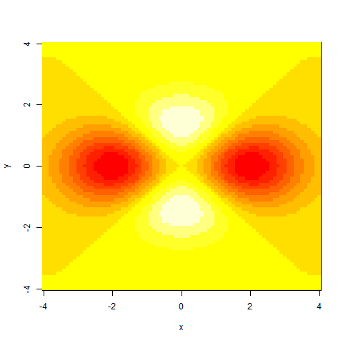
# also useful:
image( x , y , z )

persp( x , y , z )

# with plot3D package:
require(plot3D)
persp3D( x , y , z )

#
# END Example Contour-Plot
#-----------------------------------------------------



# Let's make a contour-plot of the log-likelihood function:
#
# Grid for the model parameters (recall that the model 
# is unstable for w0=0 or bsvol=0):

bsvol = seq( from=0.1/100 , to=4/100 , by=0.1/100 )
w0 = seq( from=0.05 , to=0.95 , by=0.05 )


# the following does not work, since logL does not accept 
# vectors as input; the reason is that in logL there is a line
# vol = sqrt(w0*bsvol^2+w1*ret^2) 
# which does not make sense if all w0, w1 and ret are vectors:

z = outer( bsvol , w0 , FUN = logL )          # does not work

# so let's do this with a loop:

nbs = length(bsvol)
nw = length(w0)
z = matrix( 0 , nrow=nbs , ncol=nw )
for(i in 1:nbs)
{
  for(j in 1:nw )
  {
    z[i,j] = logL( bsvol[i] , w0[j] )         # this is ok
  }
}

# let's look at the result:
contour( bsvol , w0 , z )

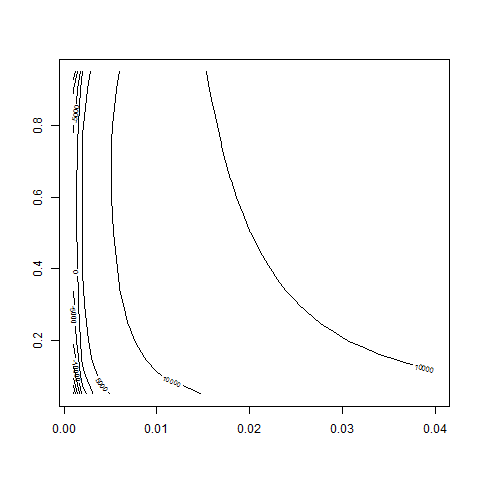
contour( bsvol , w0 , z , nlevels = 50 )

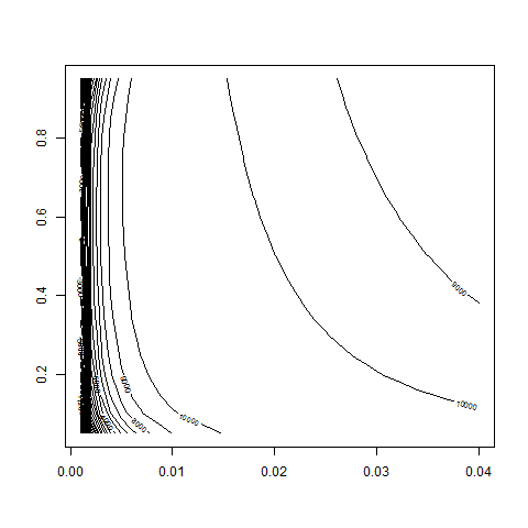
contour( bsvol , w0 , z , nlevels = 50 , zlim=c(10000,11000) )       
# eventually vary range for zlim-values

# okay, that works!!  -> we recover correct parameter values!!
# bsvol around 0.01 and w0 around 0.5


# some more pictures (would require more fine-tuning):
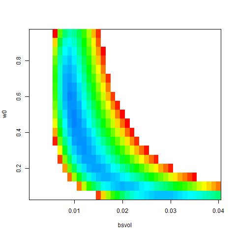
image( bsvol , w0 , z )

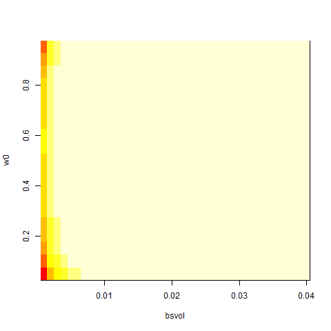
image( bsvol , w0 , z , col = rainbow(100) , zlim=c(10000,11000) )

persp( bsvol , w0 , z )

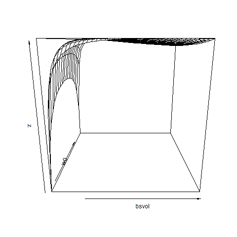
persp3D( bsvol , w0 , z )

---------------------------------------
#     ARCH(1)-Fit to DAX-Data:        #
---------------------------------------

# load DAX.txt data and generate return vector ret:

dax = read.table("C:/Users/Admin/Courses/FinancialStatistics/DAX.txt",header=TRUE,sep=";")
dax = na.omit(dax)
summary(dax)
S = dax$index
n = length(S)
ret = rep(0,n)       
for(i in 2:n)
{
  ret[i] = (S[i]-S[i-1])/S[i-1]
}
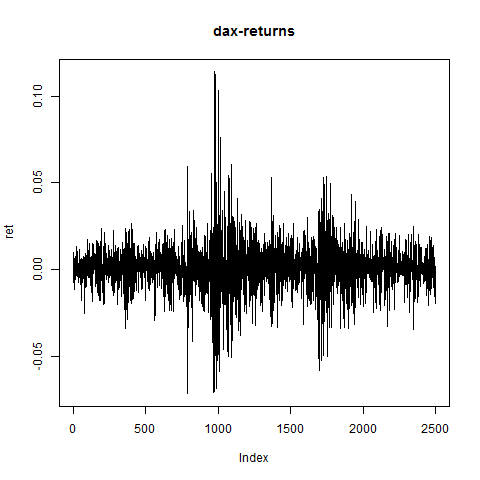
plot(ret,type="l",main="dax-returns")

#
# calculate DAX-logL and make setup for contour-plot:
#
bsvol = seq( from=0.1/100 , to=4/100 , by=0.1/100 )
w0 = seq( from=0.05 , to=0.95 , by=0.05 )
nbs = length(bsvol)
nw = length(w0)

z = matrix( 0 , nrow=nbs , ncol=nw )
for(i in 1:nbs)
{
  for(j in 1:nw )
  {
    z[i,j] = logL( bsvol[i] , w0[j] )         
  }
}

# let's look at the result:
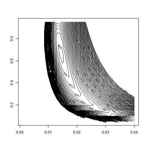
contour( bsvol , w0 , z )

contour( bsvol , w0 , z , nlevels = 50 )

contour( bsvol , w0 , z , nlevels = 50 , zlim=c(8000,10000) )

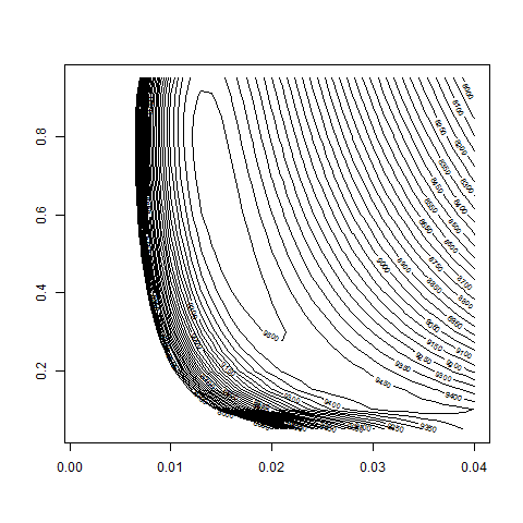
contour( bsvol , w0 , z , nlevels = 50 , zlim=c(9000,9600) )

# we take a more refined look at the region w0 = 0.5 to 0.9
# and bsvol = 1.0% to 2.0%:

bsvol = seq( from=1.0/100 , to=2.0/100 , by=0.02/100 )
w0 = seq( from=0.5 , to=0.9 , by=0.01 )
nbs = length(bsvol)
nw = length(w0)
z = matrix( 0 , nrow=nbs , ncol=nw )
for(i in 1:nbs)
{
  for(j in 1:nw )
  {
    z[i,j] = logL( bsvol[i] , w0[j] )         
  }
}

# let's look at the results:
contour( bsvol , w0 , z , nlevels = 100 , zlim=c(9000,9600) )

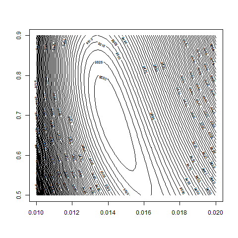
contour( bsvol , w0 , z , nlevels = 100 , zlim=c(9500,9550) )

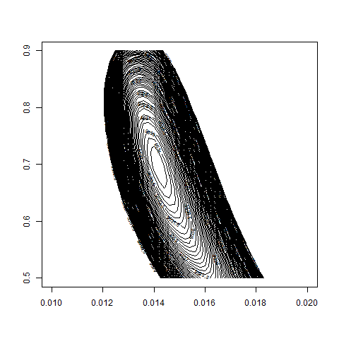
max(z)                             # 9534.98
logL( bsvol=sd(ret) , w0=0.72 )    # 9534.64
sd(ret)                            # 1.39%

# thus: maximum approximately at 
# bsvol = sd(ret) = 1.39% and w0 = 0.72



# Before we redo the calculations for SPX and GE, we code 
# a small function GetZ which sets up the matrix z for 
# the contour-plots:

GetZ = function( x , y )
{
  nx = length(x)
  ny = length(y)
  z = matrix( 0 , nrow=nx , ncol=ny )
  for(i in 1:nx)
  {
    for(j in 1:ny)
    {
      z[i,j] = logL(x[i],y[j])
    }
  }
  return(z)
}



---------------------------------------
#     ARCH(1)-Fit to S&P500-Data:     #
---------------------------------------

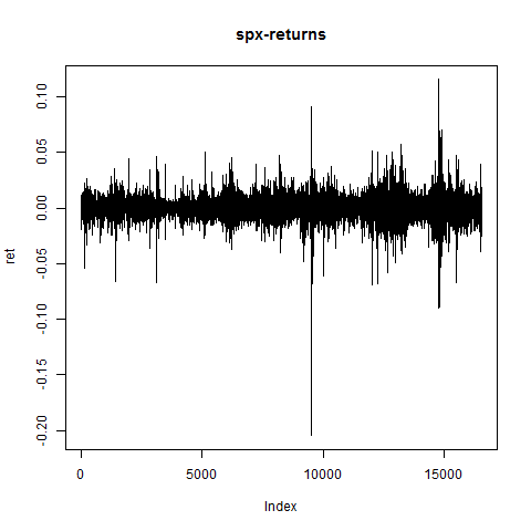
# load SPX.txt data and generate return vector ret:

spx = read.table("C:/Users/Admin/Courses/FinancialStatistics/SPX.txt",header=TRUE,sep=";")
head(spx)
summary(spx)     # no NA's
S = spx[,2]
n = length(S)
ret = rep(0,n)       
for(i in 2:n)
{
  ret[i] = (S[i]-S[i-1])/S[i-1]
}
plot(ret,type="l",main="spx-returns")   # returns look ok

# compute spx-logL and make setup for contour-plot:

bsvol = seq( from=0.1/100 , to=4/100 , by=0.1/100 )
w0 = seq( from=0.05 , to=0.95 , by=0.05 )

z = GetZ( bsvol , w0 )


# let's look at the results:

contour( bsvol , w0 , z )

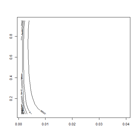
contour( bsvol , w0 , z , nlevels = 50 )

contour( bsvol , w0 , z , nlevels = 50 , zlim=c(60000,80000) )

contour( bsvol , w0 , z , nlevels = 100 , zlim=c(60000,80000) )

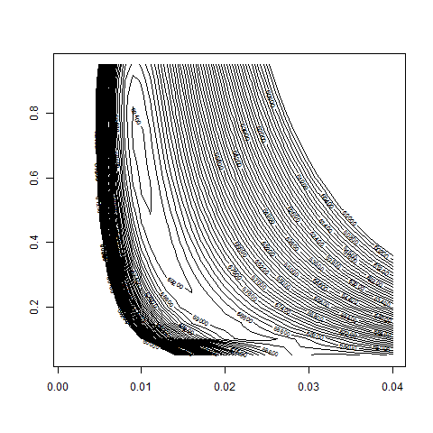
# we take a more refined look at the region w0 = 0.5 to 0.9
# and bsvol = 0.5% to 1.5%:

bsvol = seq( from=0.5/100 , to=1.5/100 , by=0.02/100 )
w0 = seq( from=0.5 , to=0.9 , by=0.01 )

z = GetZ( bsvol , w0 )

contour( bsvol , w0 , z , nlevels = 100 , zlim=c(60000,80000) )

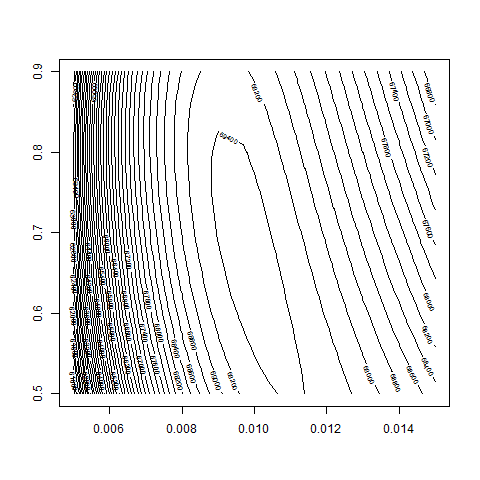
contour( bsvol , w0 , z , nlevels = 100 , zlim=c(69000,70000) )

max(z)                             # 69471.9
logL( bsvol=sd(ret) , w0=0.69 )    # 69472.17
sd(ret)                            # 0.97%

# thus: maximum approximately at 
# bsvol = sd(ret) = 0.97% and w0 = 0.69



---------------------------------------
#     ARCH(1)-Fit to GE-Data:         #
---------------------------------------

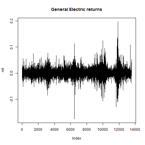
# load GE.txt data and generate return vector ret:

ge = read.table("C:/Users/Admin/Courses/FinancialStatistics/GE.txt",header=TRUE,sep=";")
head(ge)
summary(ge)     # no NA's
S = ge[,2]
n = length(S)
ret = rep(0,n)       
for(i in 2:n)
{
  ret[i] = (S[i]-S[i-1])/S[i-1]
}
plot(ret,type="l",main="General Electric returns")   
# returns look ok:

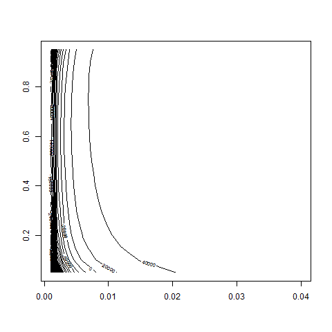
# compute GE-logL and make setup for contour-plot:

bsvol = seq( from=0.1/100 , to=4/100 , by=0.1/100 )
w0 = seq( from=0.05 , to=0.95 , by=0.05 )

z = GetZ( bsvol , w0 )


# let's look at the result:

contour( bsvol , w0 , z )

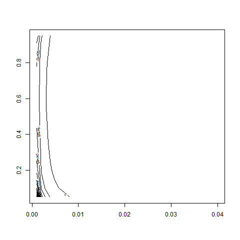
contour( bsvol , w0 , z , nlevels = 50 )

contour( bsvol , w0 , z , nlevels = 50 , zlim=c(40000,50000) )

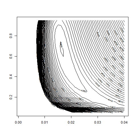
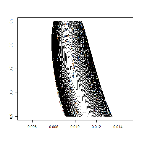
# we take a more refined look at the region w0 = 0.5 to 0.9
# and bsvol = 1.0% to 2.0%:

bsvol = seq( from=1.0/100 , to=2.0/100 , by=0.02/100 )
w0 = seq( from=0.5 , to=0.9 , by=0.01 )

z = GetZ( bsvol , w0 )

contour( bsvol , w0 , z , nlevels = 50 , zlim=c(40000,50000) )

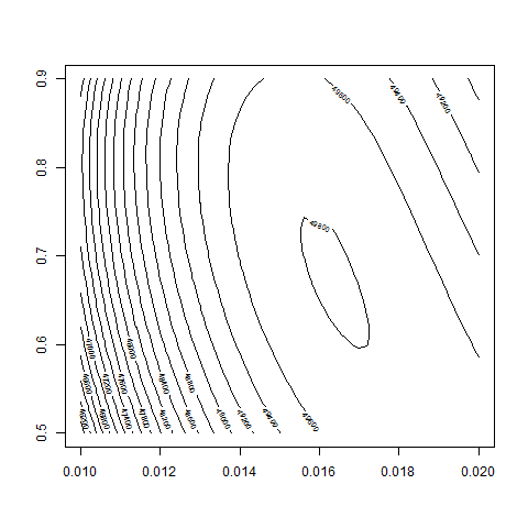
contour( bsvol , w0 , z , nlevels = 100 , zlim=c(49500,50000) )

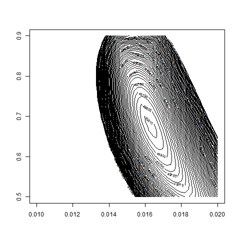
max(z)                             # 49811.81
logL( bsvol=sd(ret) , w0=0.68 )    # 49811.89
sd(ret)                            # 1.62%

# thus: maximum approximately at 
# bsvol = sd(ret) = 1.62% and w0 = 0.68